Multilayer Perceptrons and Backpropagation

Deep Learning: Multilayer Perceptrons and Backpropagation

Here is my Deep Learning Full Tutorial!

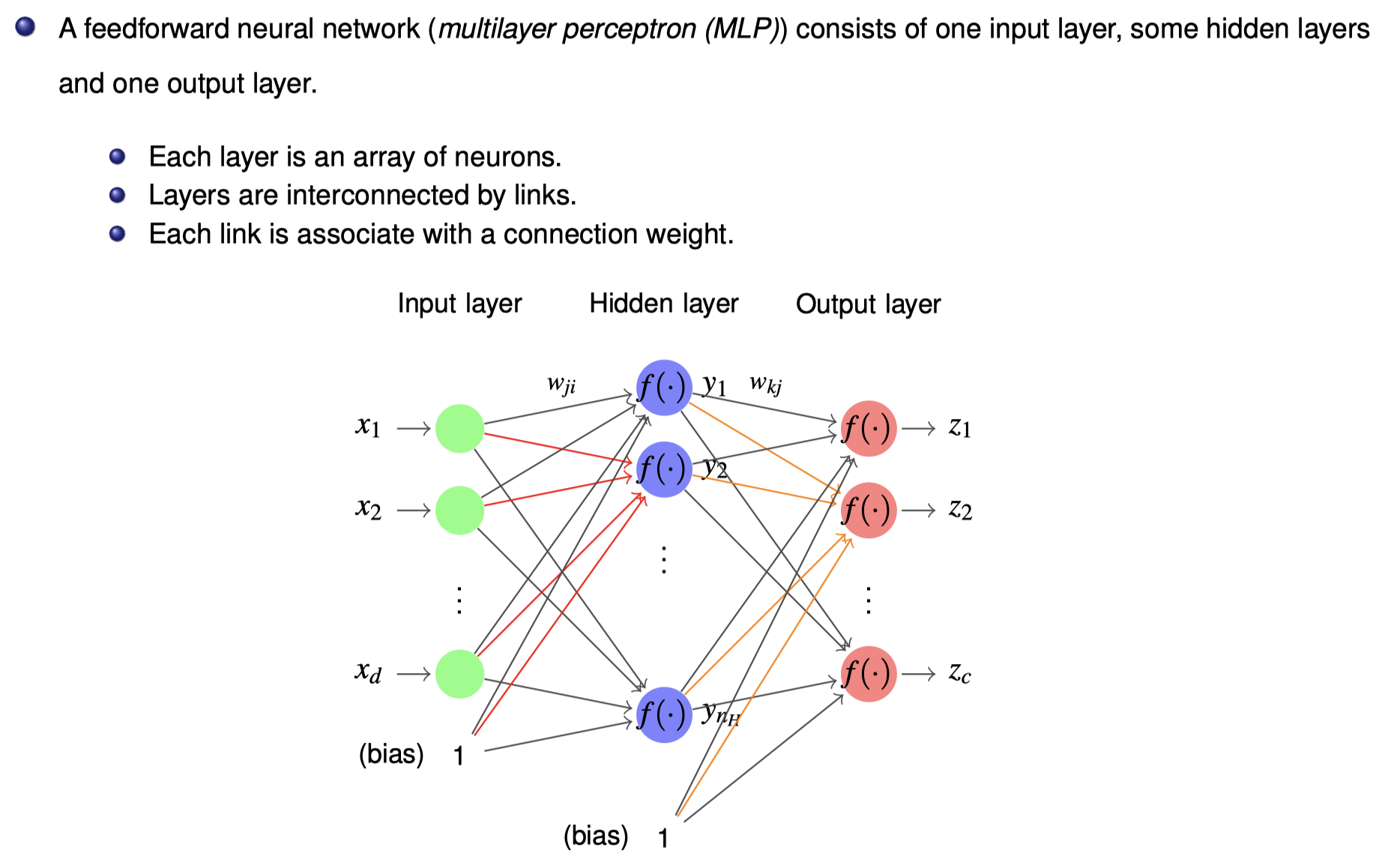
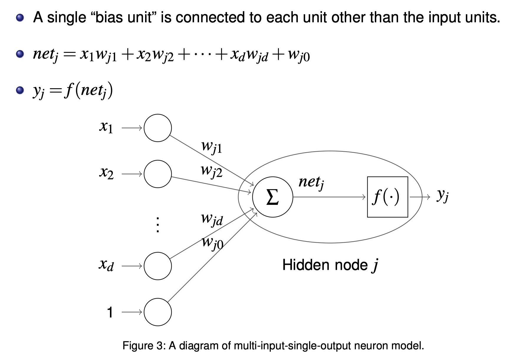
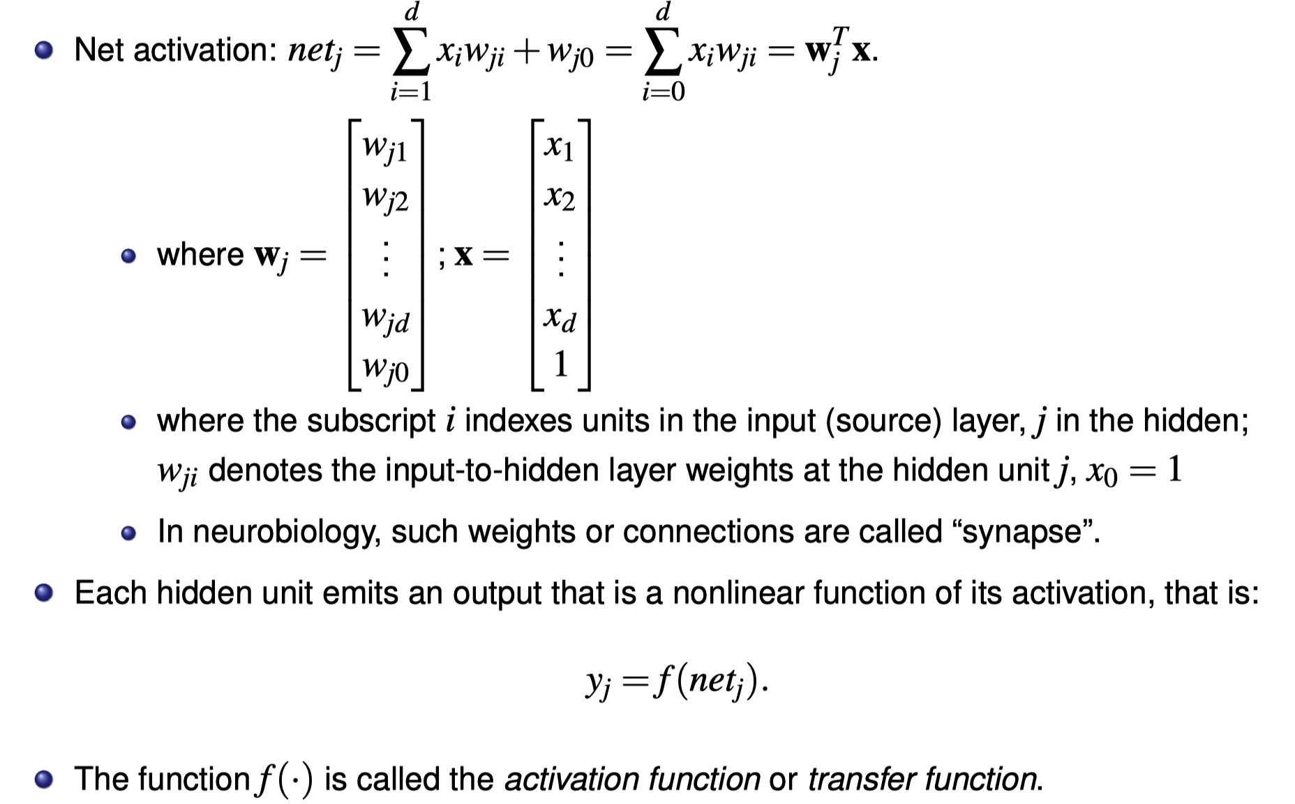
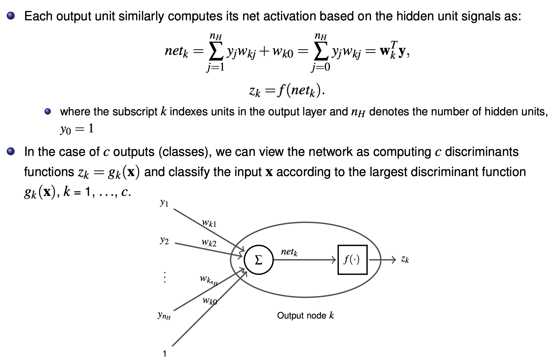
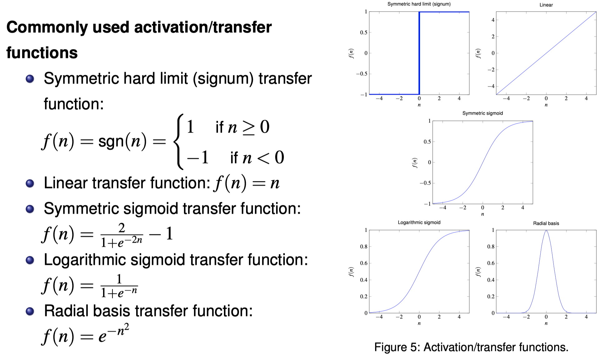
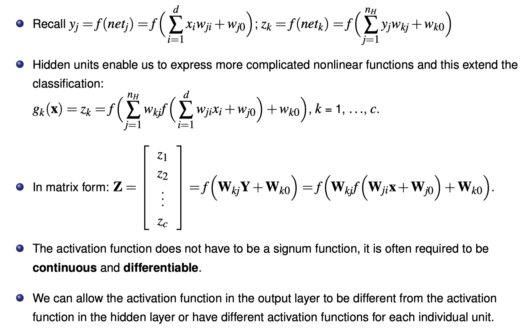
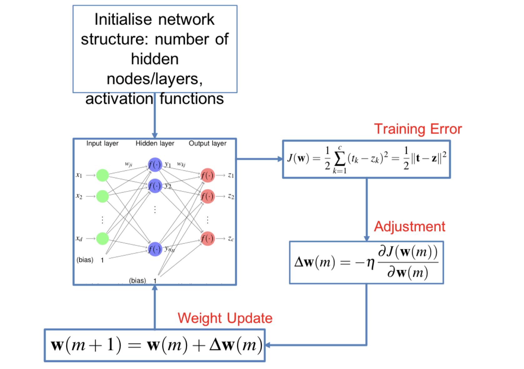
Feedforward Neural Networks

Feedforward Neural Networks Python code

# Feedforward Neural Networks
import numpy as np
from prettytable import PrettyTable
import math
np.set_printoptions(suppress=True)

def log_sigmod(input):
    return 1. / (1. + np.exp(-input))

def d_log_sigmod(input):
    # e^(-x)/(1+e^(-x))^2
    return np.exp(-input)/((1+np.exp(-input))*(1+np.exp(-input)))


def sym_sigmod(input):
    ex = np.exp(input)
    enx = np.exp(-input)
    return (ex - enx) / (ex + enx)

def d_sym_sigmod(input):
    # 4e^(-2x)/(1+e^(-2x))^2
    return 4*np.exp(-2*input)/((1+np.exp(-2*input))*(1+np.exp(-2*input)))

def linear(input):
    return input

def cost(y_pred,y):
    return 0.5*(y_pred-y)*(y_pred-y)

def d_cost(y_pred,y):
    return y_pred - y

# input data
X = [[0.4,-0.4]]
w1 = [
    [5,3],
    [-5,-5],
    [5,-2]
    ]
b1 = [-1,-3,4]
w2 = [
    [5,-1,-5],
    [5,1,-1]
    ]
b2 = [-4,1]
# input layer to hidden layer
y1 = sym_sigmod(np.dot(X,np.transpose(w1)) + b1)
z = np.dot(y1,np.transpose(w2)) + b2
print(np.dot(X,np.transpose(w1)) + b1)
print(np.round(y1,4))
print(np.round(z,4))
print(np.sum(np.power(z[0] - np.array([-5,5]),2)/2))

Output

[[-0.2 -3.   6.8]]
[[-0.1974 -0.9951  1.    ]]
[[-8.9918 -1.9819]]
32.34093671219539

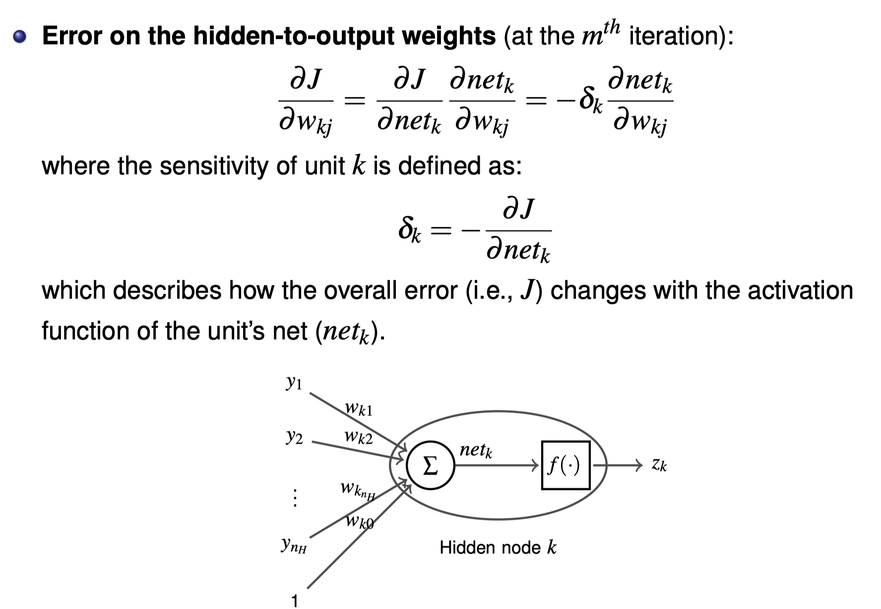
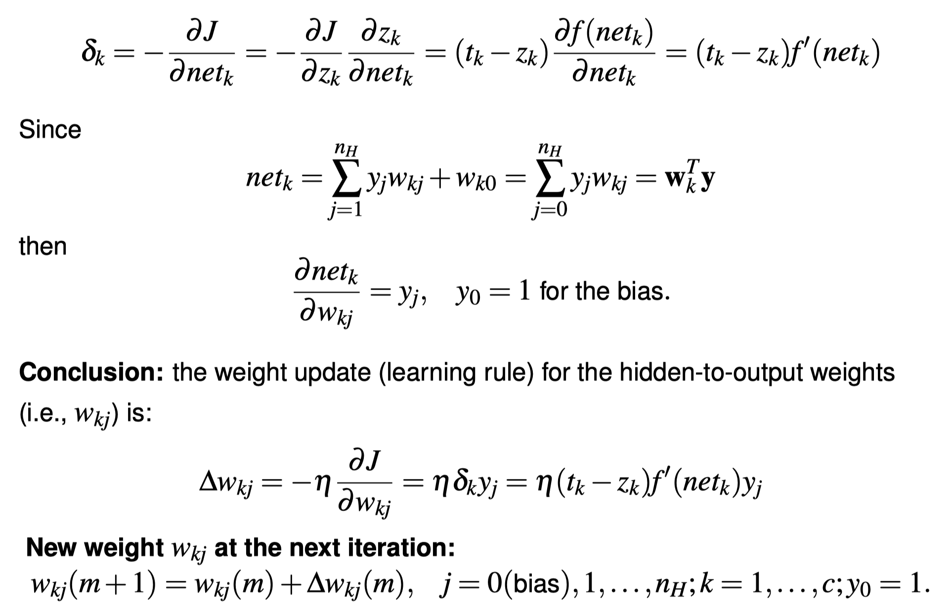
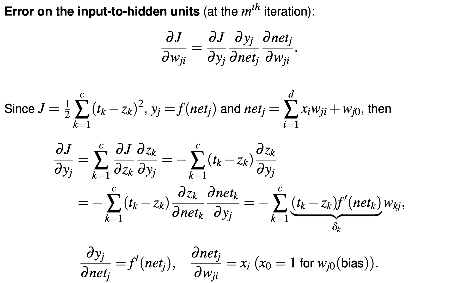
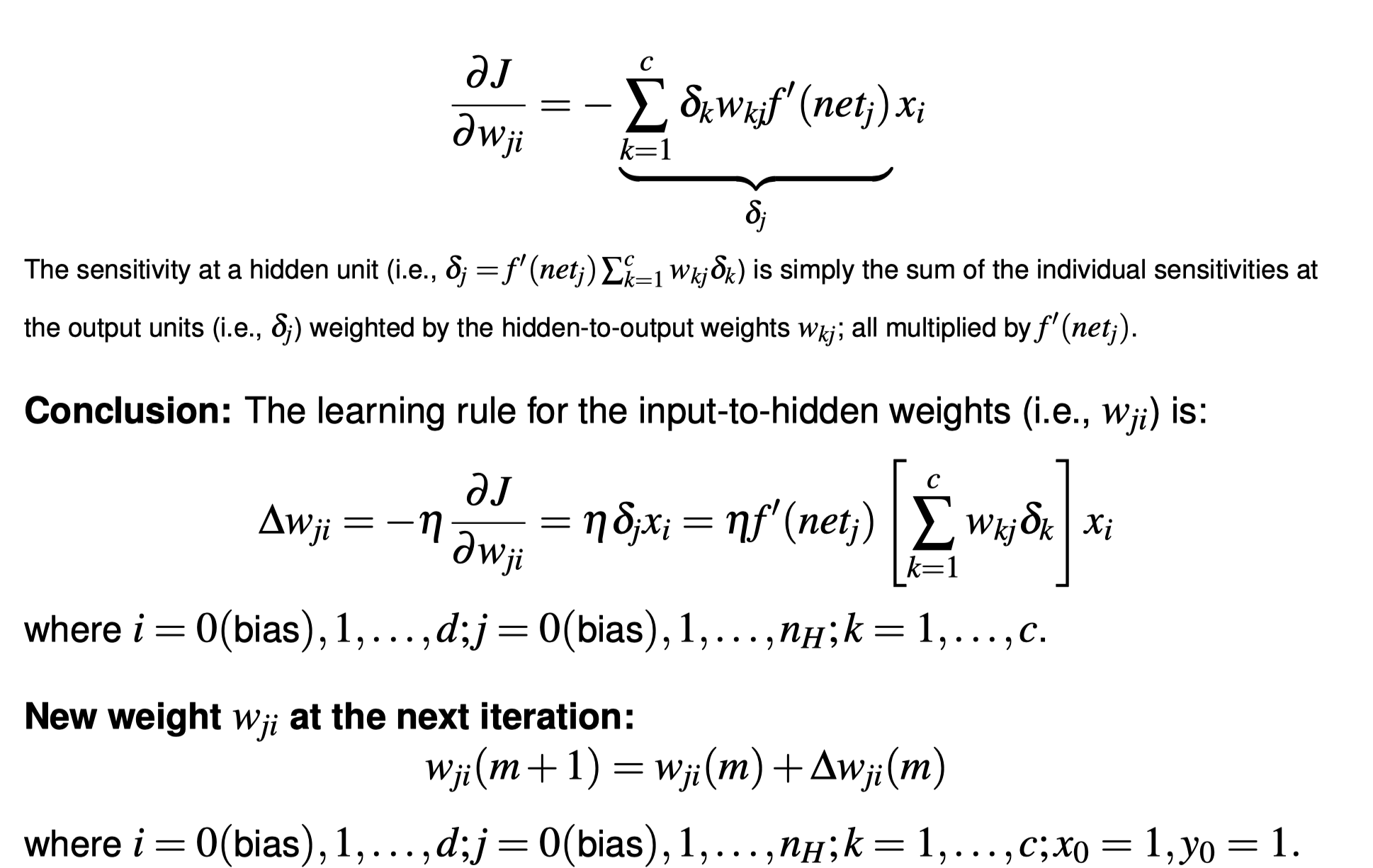
Backpropagation Algorithm

Backpropagation Algorithm Python Code

# Backpropagation Algorithm
x = [0.4,-0.4]
net = -1.0633
y_pred = -8.9918
y = -5
m = -0.1974

# learning rate
n = 0.3
# d_m = ∂cost/∂m = ∂cost/∂f(mx+b) * ∂f(mx+b)/∂(mx+b) * ∂(mx+b)/∂m
d_m = d_cost(y_pred,y)*d_sym_sigmod(net)*net
m_new = -n*d_m + m
result = np.round([(net,y,y_pred,d_cost(y_pred,y),1,net,d_m,m_new)],4)


pt = PrettyTable(('net','y','y_pred','∂cost/∂f(wx+b)','∂f(wx+b)/∂(wx+b)','∂(wx+b)/∂w','d_m','m_new'))
for row in result: pt.add_row(row)
print(pt)

y_2 = -2
m_2 = 1.6
w = 5
a = 0.4

# d_w = ∂cost/∂w = ∂cost/∂f(m*g(wx+b)+b) * ∂f(m*g(wx+b)+b)/∂(m*g(wx+b)+b) * ∂(m*g(wx+b)+b)/∂g(wx+b) * ∂(g(wx+b))/∂(wx+b) * ∂(wx+b)/∂w
d_w = d_cost(y_pred,y)*m_2 * d_sym_sigmod(-0.2) * x[0]
w_new = -n*d_w + w
result = np.round([(net,y,y_pred,d_cost(y_pred,y),d_sym_sigmod(net),m_2,d_sym_sigmod(a),x[0],d_w,w_new)],4)

pt = PrettyTable(('net','y','y_pred','∂cost/∂f(m*g(wx+b)+b)','∂f(m*g(wx+b)+b)/∂(m*g(wx+b)+b)','∂(m*g(wx+b)+b)/∂g(wx+b)','∂(g(wx+b))/∂(wx+b)','∂(wx+b)/∂w','d_w','w_new'))
for row in result: pt.add_row(row)
print(pt)

Output

+---------+------+---------+----------------+------------------+------------+--------+---------+
|   net   |  y   |  y_pred | ∂cost/∂f(wx+b) | ∂f(wx+b)/∂(wx+b) | ∂(wx+b)/∂w |  d_m   |  m_new  |
+---------+------+---------+----------------+------------------+------------+--------+---------+
| -1.0633 | -5.0 | -8.9918 |    -3.9918     |       1.0        |  -1.0633   | 1.6161 | -0.6822 |
+---------+------+---------+----------------+------------------+------------+--------+---------+
+---------+------+---------+-----------------------+--------------------------------+-------------------------+--------------------+------------+---------+--------+
|   net   |  y   |  y_pred | ∂cost/∂f(m*g(wx+b)+b) | ∂f(m*g(wx+b)+b)/∂(m*g(wx+b)+b) | ∂(m*g(wx+b)+b)/∂g(wx+b) | ∂(g(wx+b))/∂(wx+b) | ∂(wx+b)/∂w |   d_w   | w_new  |
+---------+------+---------+-----------------------+--------------------------------+-------------------------+--------------------+------------+---------+--------+
| -1.0633 | -5.0 | -8.9918 |        -3.9918        |             0.3808             |           1.6           |       0.8556       |    0.4     | -2.4552 | 5.7366 |
+---------+------+---------+-----------------------+--------------------------------+-------------------------+--------------------+------------+---------+--------+

RBF network output unit Python Code

# RBF network output unit
w = [-2.5027,-2.5027]
b = 2.8413
z = np.dot(np.transpose(y),np.transpose([w])) + b
np.set_printoptions(suppress=True)
print(z)

Output

[[-0.00010361]
[ 0.99991625]
[ 0.99991625]
[-0.00010361]]

Continue Python Code

# m * w = z, get w
m = np.transpose(np.append(y,np.array([[1,1,1,1]]),axis=0))
z = np.array([[0,1,1,0]])
print('Z:\n',z)
print('Y:\n',m)
w = np.dot(np.dot(np.linalg.inv(np.dot(np.transpose(m),m)),np.transpose(m)),np.transpose(z))
print('W:\n',w)

Output

Z:
[[0 1 1 0]]
Y:
[[1.         0.13533528 1.        ]
[0.36787944 0.36787944 1.        ]
[0.36787944 0.36787944 1.        ]
[0.13533528 1.         1.        ]]
W:
[[-2.5026503 ]
[-2.5026503 ]
[ 2.84134719]]