Deep Discriminative Neural Networks

Deep Learning: Deep Discriminative Neural Networks

Here is my Deep Learning Full Tutorial!

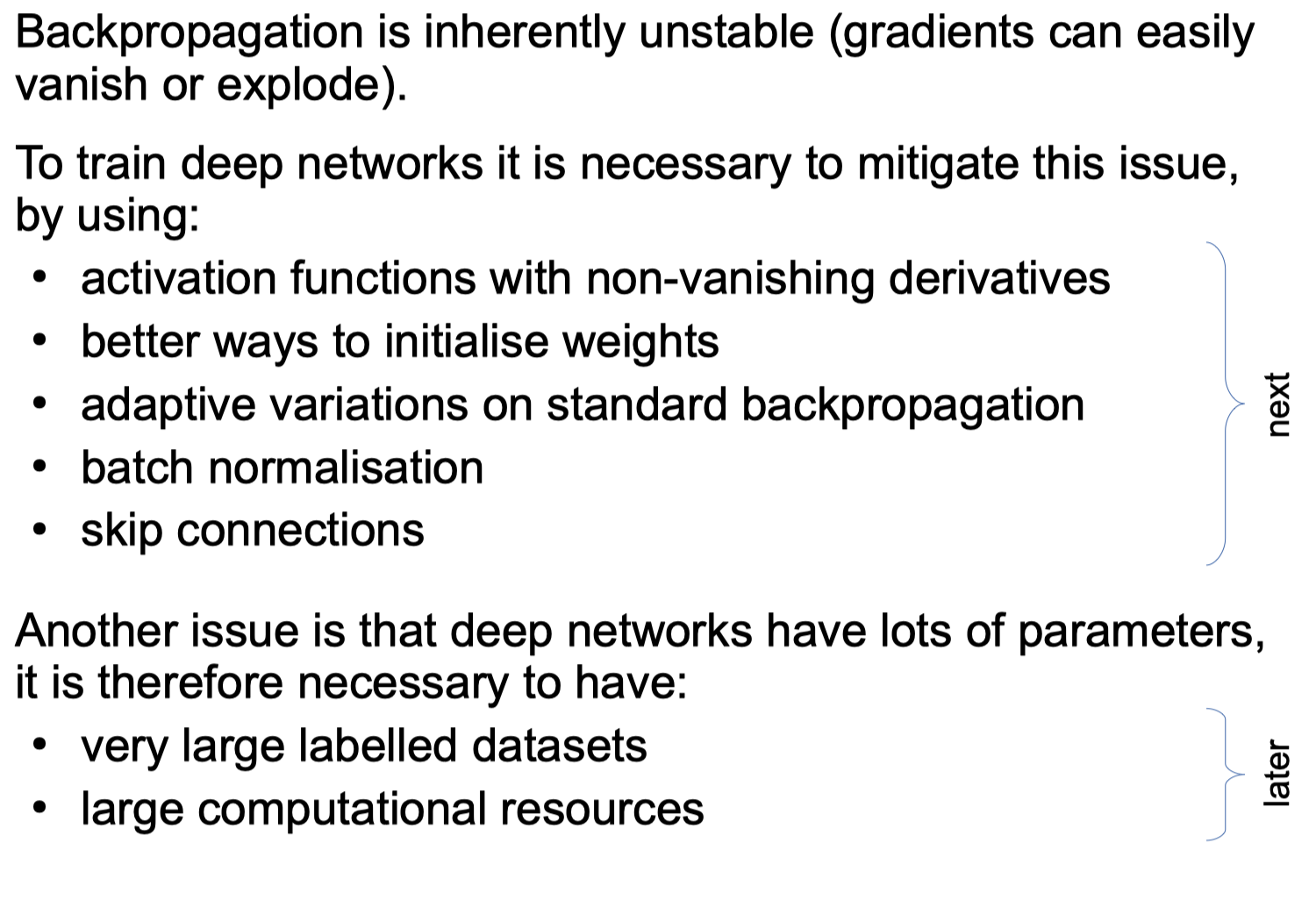
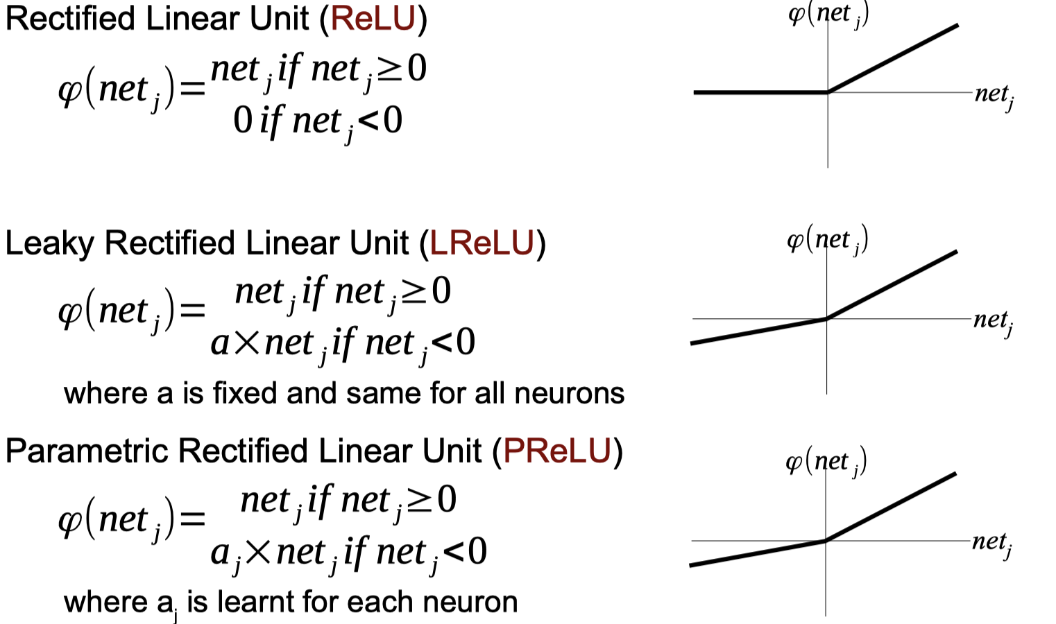
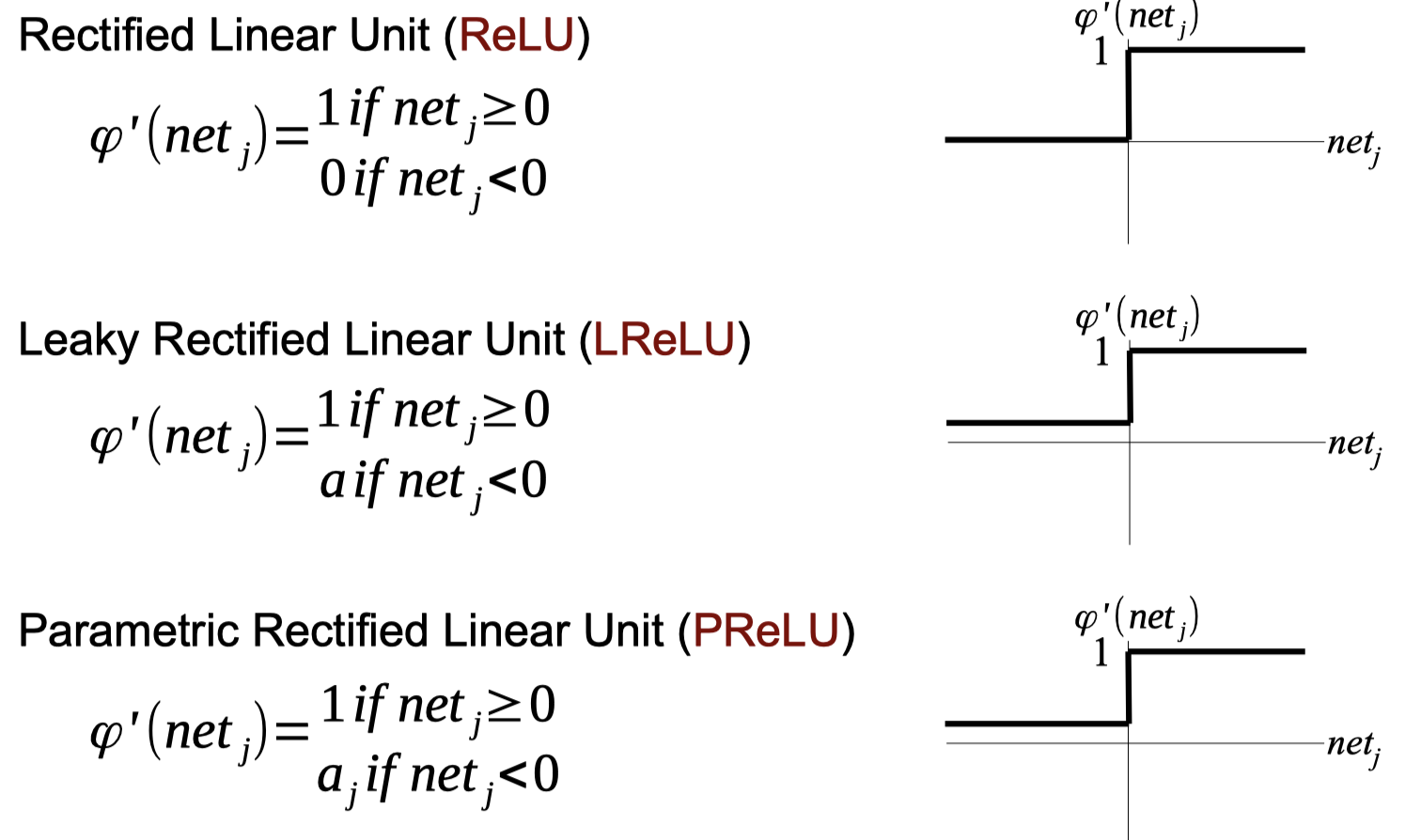
Activation Functions with Non-Vanishing Derivatives

Activate Functions Python code

# Activate Functions
import numpy as np


def relu(input):
    return (np.abs(input) + input)/2
def l_relu(input):
    return np.where(input > 0, input, input * 0.1) 

def tanh(input):
    ex = np.exp(input)
    enx = np.exp(-input)
    return (ex - enx) / (ex + enx)

def d_tanh(input):
    # 4e^(-2x)/(1+e^(-2x))^2
    return 4*np.exp(-2*input)/((1+np.exp(-2*input))*(1+np.exp(-2*input)))

def heaviside(input):
    threshold = 0.1
    return np.heaviside(input-threshold,0.5) 

net = [[1,0.5,0.2],[-1,-0.5,-0.2],[0.1,-0.1,0]]
print(heaviside(np.array(net)))

Output

[[1.  1.  1. ]
[0.  0.  0. ]
[0.5 0.  0. ]]

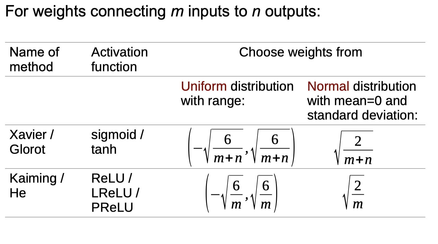
Better Ways to Initialise Weights

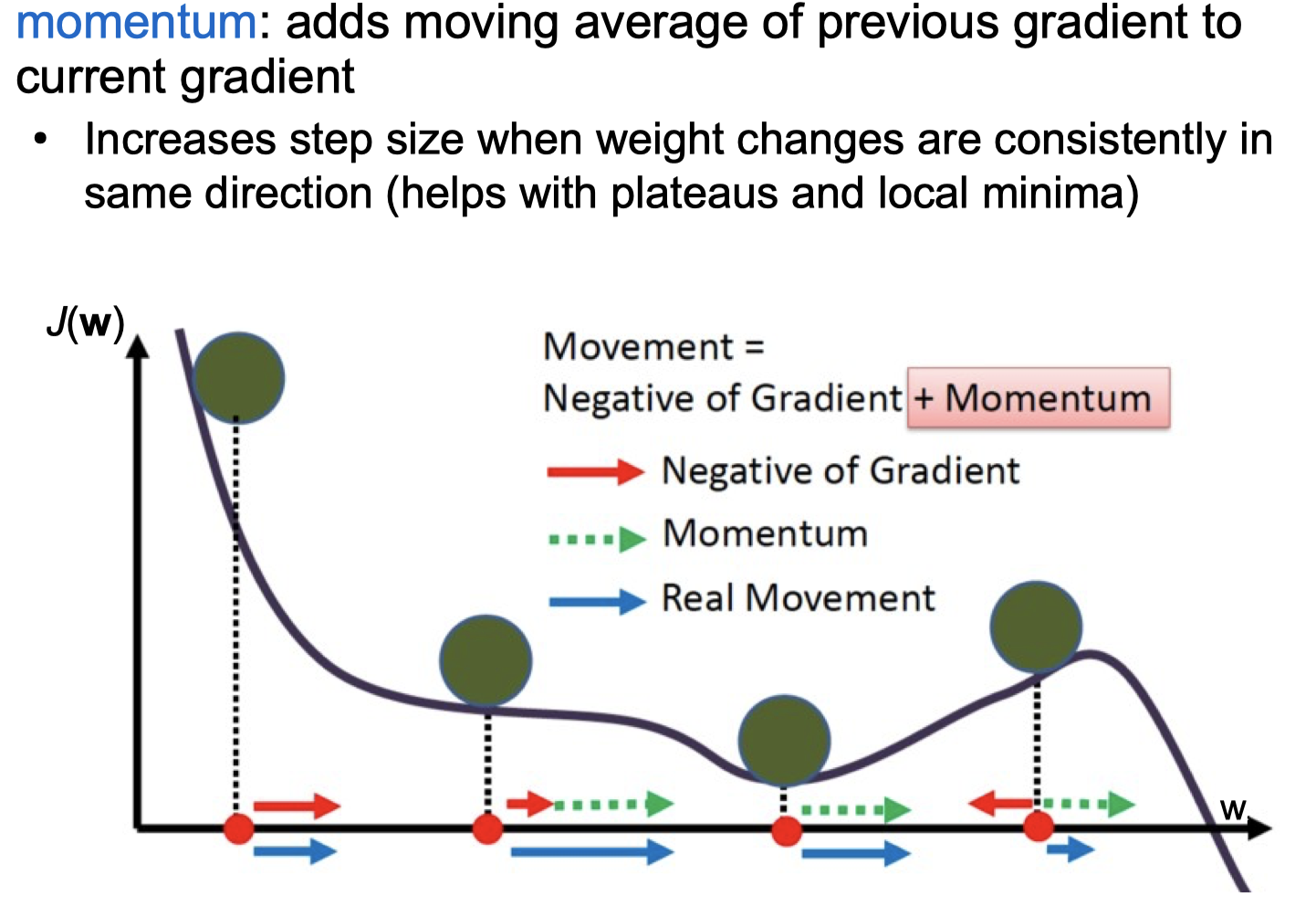
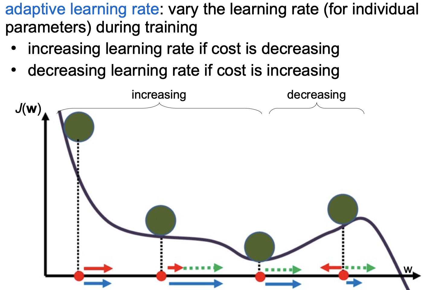
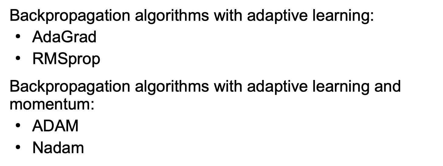
Adaptive Versions of Backpropagation

Batch Normalisation

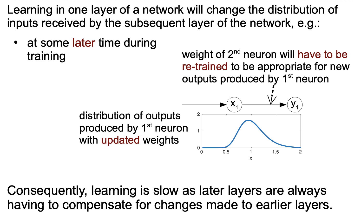
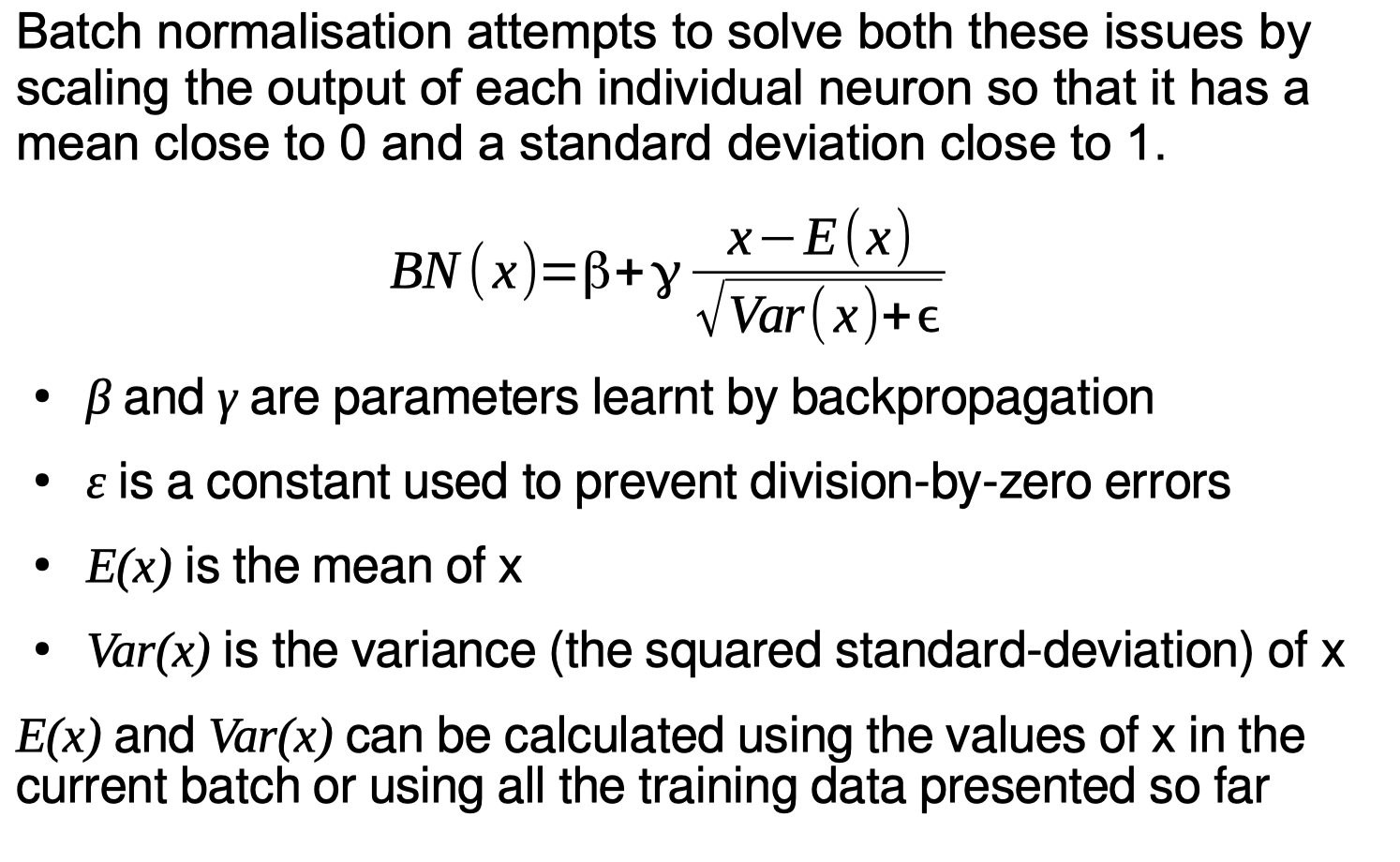
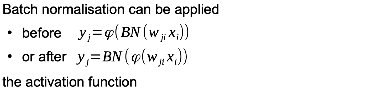
Batch normalisation

# Batch normalisation
X = [
    [[-0.3,-0.3,-0.8],[0.7,0.6,0.5],[-0.4,0.2,-0.3]],
    [[-0.5,0.1,0.8],[-0.5,-0.6,0],[0.7,-0.5,0.6]],
    [[0.8,-0.2,0.7],[0.4,0.0,0.0],[0.0,0.1,-0.6]]

    ]


def batch_normal(input):
    input = np.array(input)
    # β = 0
    a = 0.1
    # γ = 1
    b = 0.4
    # ε = 0.1
    c = 0.2
    (m,n) = np.shape(input[0])
    for x in range(m):
        for y in range(n):
            temp = np.copy(input[:,x,y])
            for i in range(len(input)):
                # the function 
                input[i,x,y] = a + b*(temp[i] - np.mean(temp))/(np.sqrt(np.var(temp)+c))
    return input
print(np.round(batch_normal(X),4))

Output

[[[-0.0654 -0.0393 -0.3819]
[ 0.3949  0.4618  0.3638]
[-0.2136  0.2962 -0.018 ]]

[[-0.1756  0.2951  0.3643]
[-0.3128 -0.2618 -0.0319]
[ 0.4764 -0.2188  0.5128]]

[[ 0.5409  0.0443  0.3177]
[ 0.218   0.1    -0.0319]
[ 0.0373  0.2226 -0.1949]]]

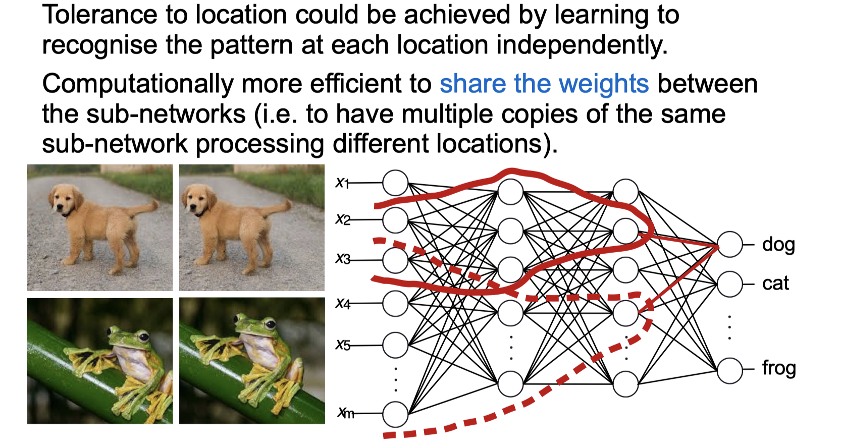
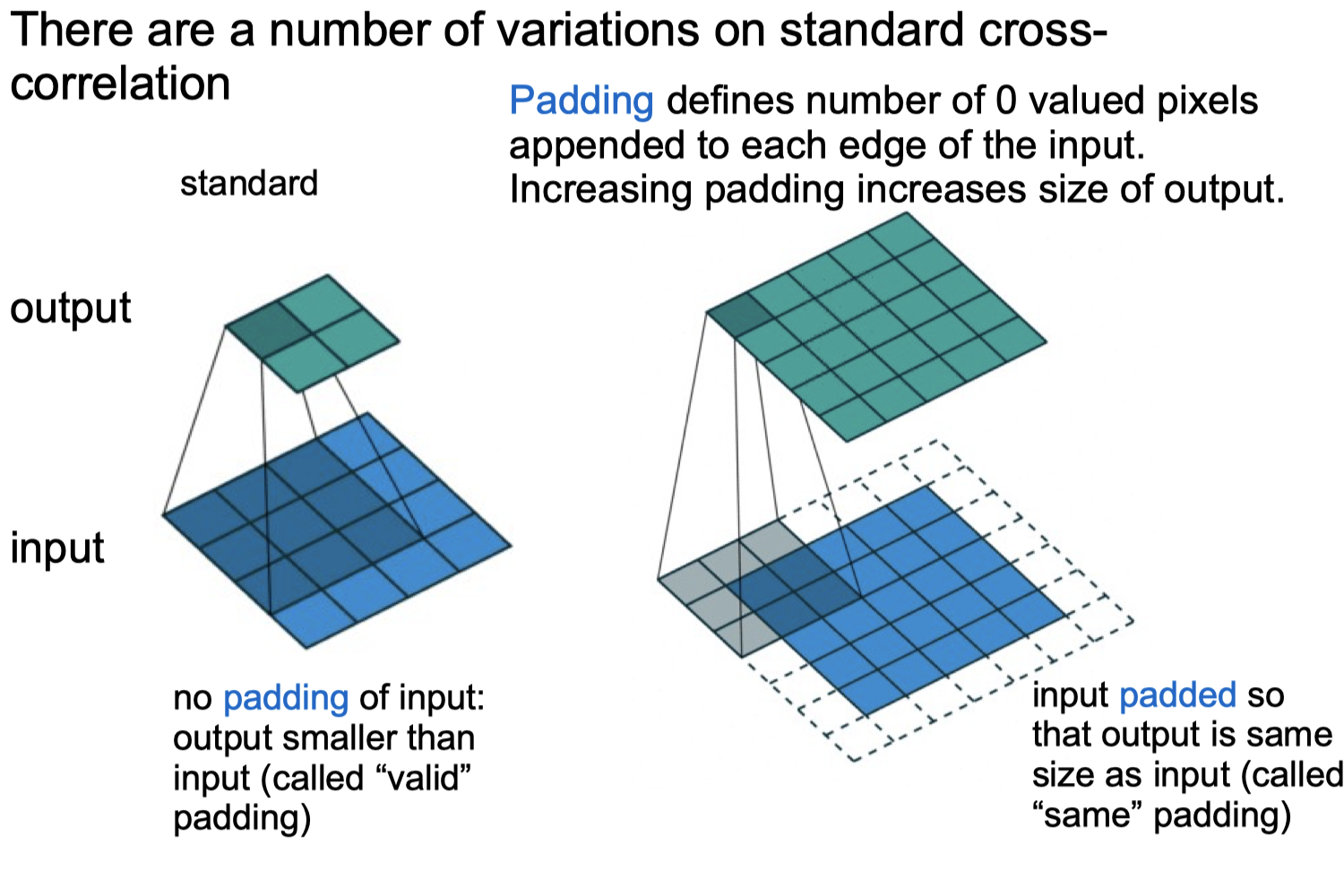
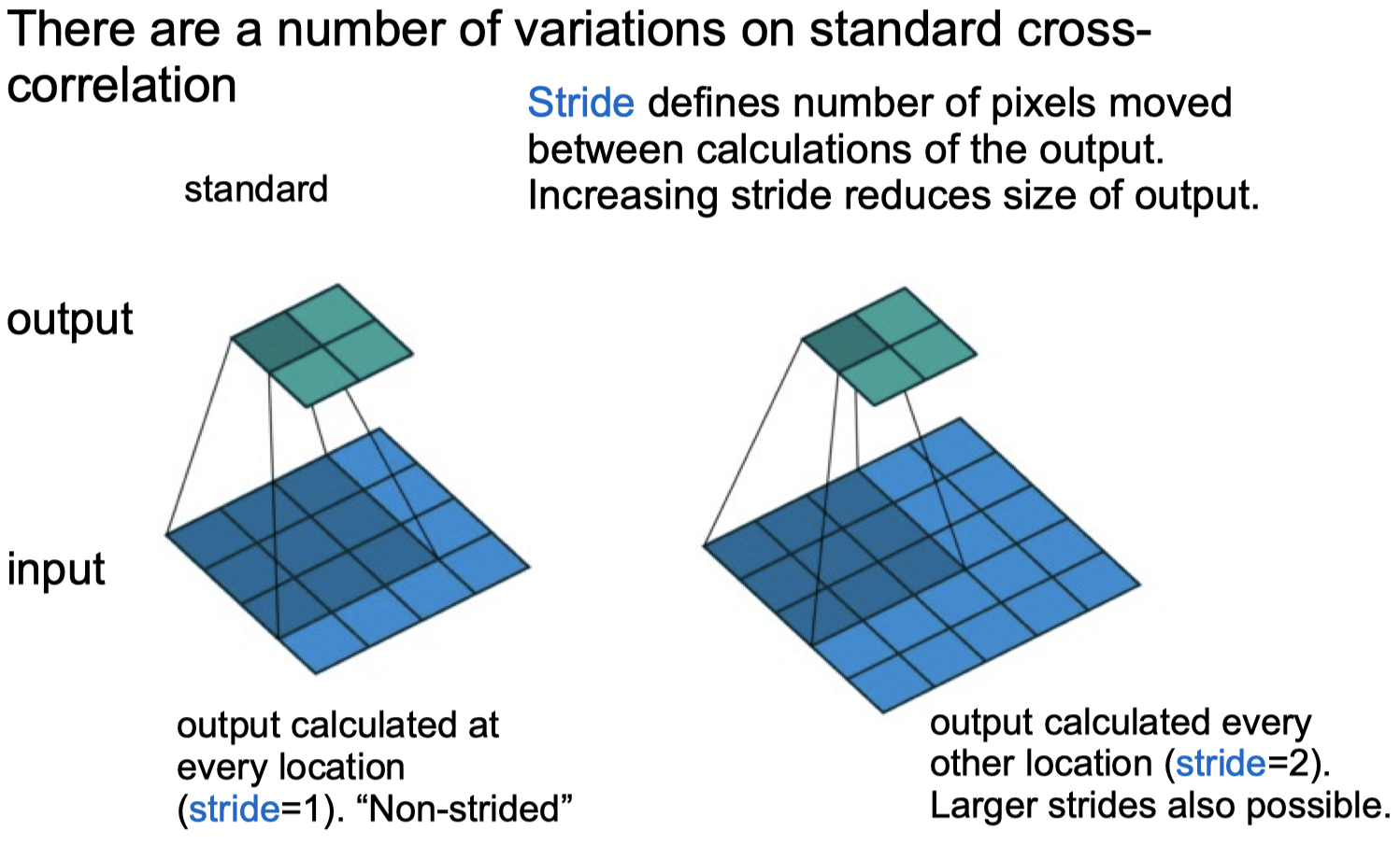
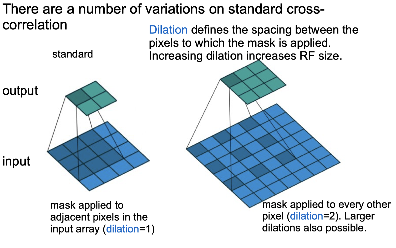
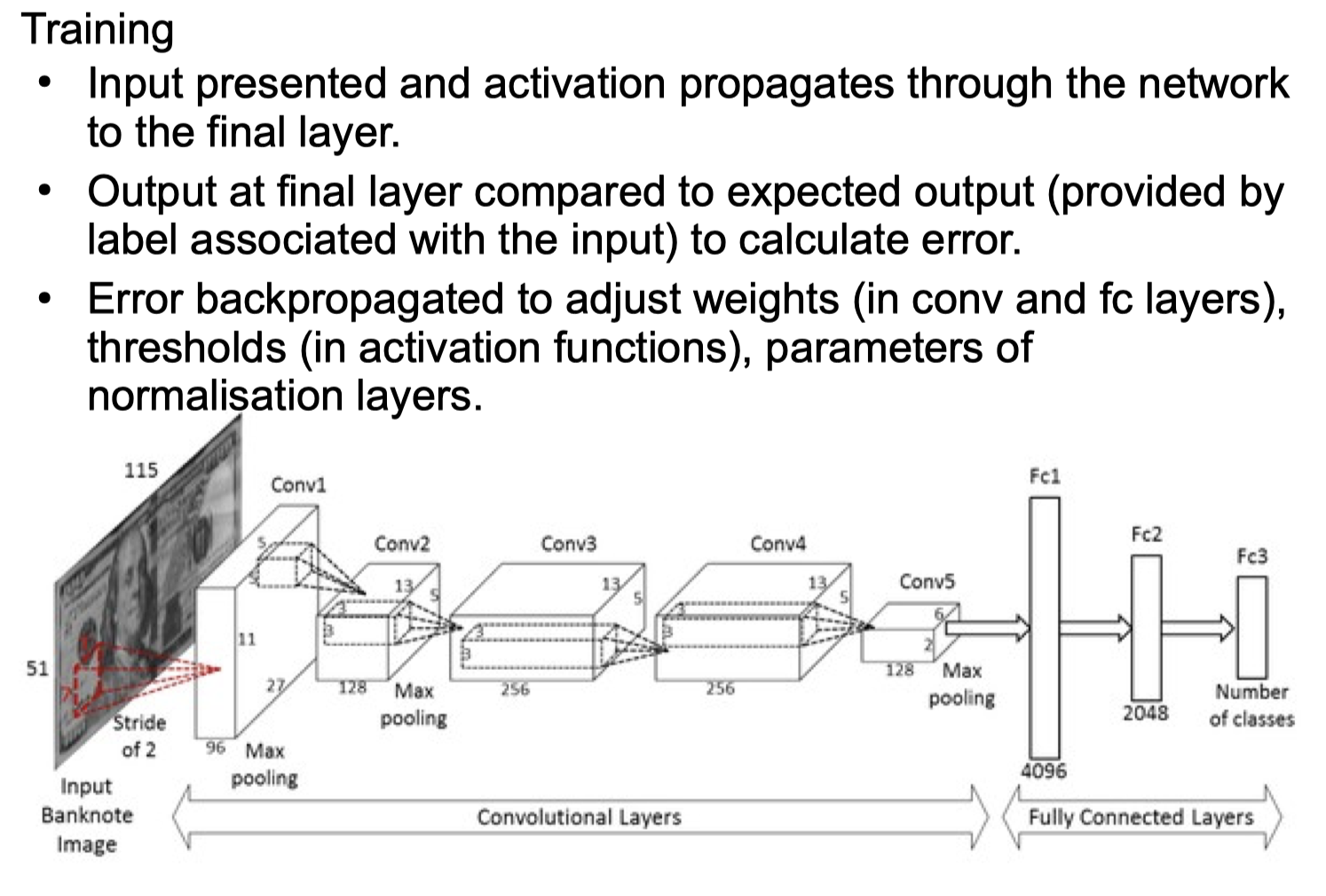
Convolutional Neural Networks

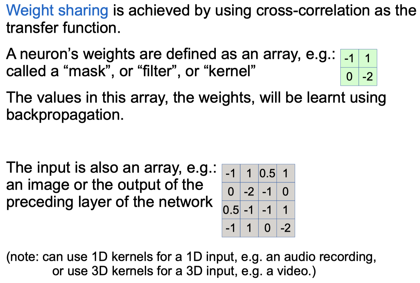
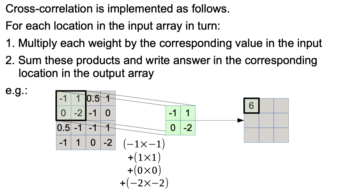
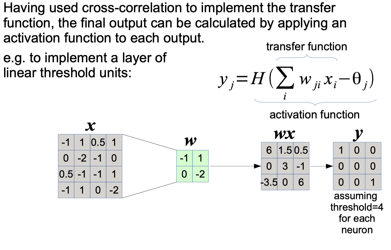
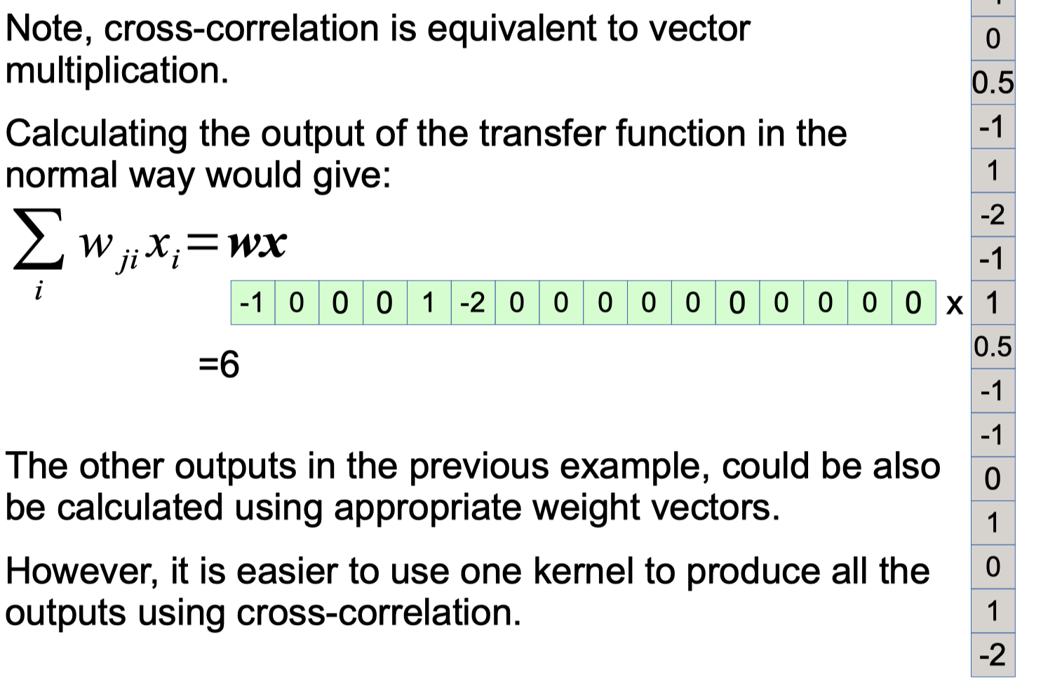
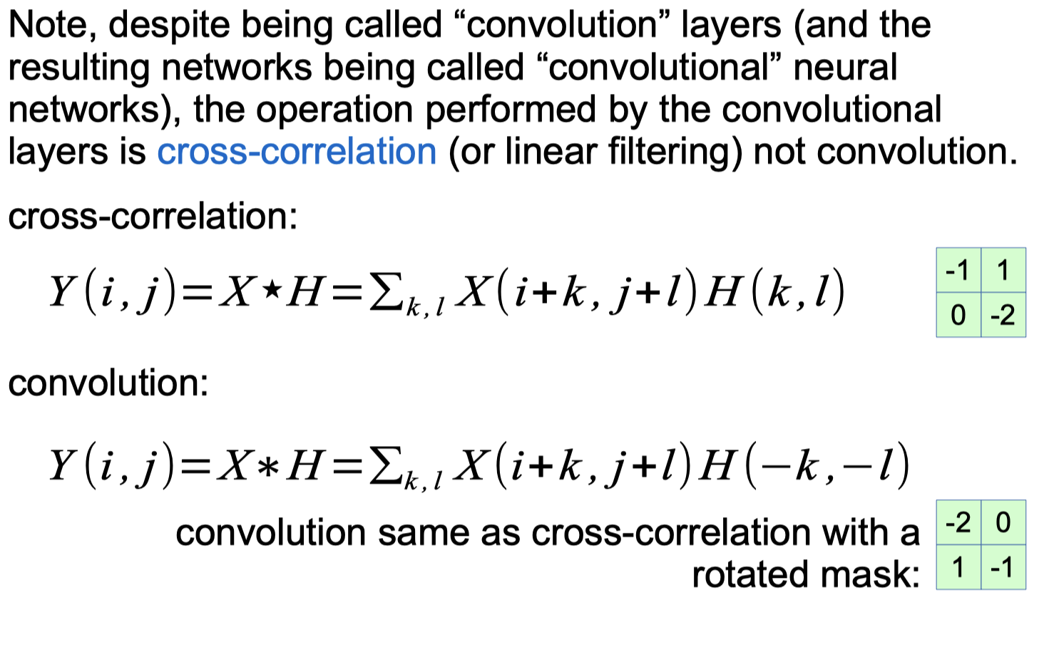
Convolutional Neural Networks Forward python code

# Convolutional Neural Networks Forward
import torch
X = [
    [[0.2,1,0],
    [-1,0,-0.1],
    [0.1,0,0.1]],
    [[1,0.5,0.2],
    [-1,-0.5,-0.2],
    [0.1,-0.1,0]]
]
H = [
    [[1,-0.1],
    [1,-0.1]],
    [[0.5,0.5],
    [-0.5,-0.5]]
]           

x = torch.tensor([X])
y = torch.tensor([H])
print(torch.nn.functional.conv2d(x,y,stride=1,padding=0, dilation=1))

Output

tensor([[[[ 0.6000,  1.7100],
        [-1.6500, -0.3000]]]])

CNN output dimension

inputDim = 200
maskDim = 5
padding = 0
stride = 1
chanel = 40
outputDim = 1 + (inputDim - maskDim + 2*padding)/stride 
print('Dimension:',outputDim,'x',outputDim,'x',chanel)

Output

Dimension: 196.0 x 196.0 x 40

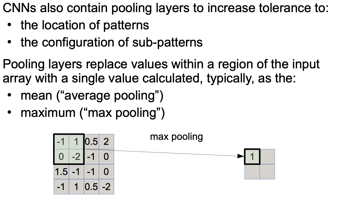
Pooling Layers

avg pooling, max pooling python code

# avg pooling, max pooling
X = [[0.2,1,0,0.4],[-1,0,-0.1,-0.1],[0.1,0,-1,-0.5],[0.4,-0.7,-0.5,1]]
x = torch.tensor([[X]])
print(torch.nn.functional.avg_pool2d(x,kernel_size =[2,2],stride=2,padding=0))
print(torch.nn.functional.max_pool2d(x,kernel_size =[3,3],stride=1,padding=0))

Output

tensor([[[[ 0.0500,  0.0500],
        [-0.0500, -0.2500]]]])
tensor([[[[1.0000, 1.0000],
        [0.4000, 1.0000]]]])

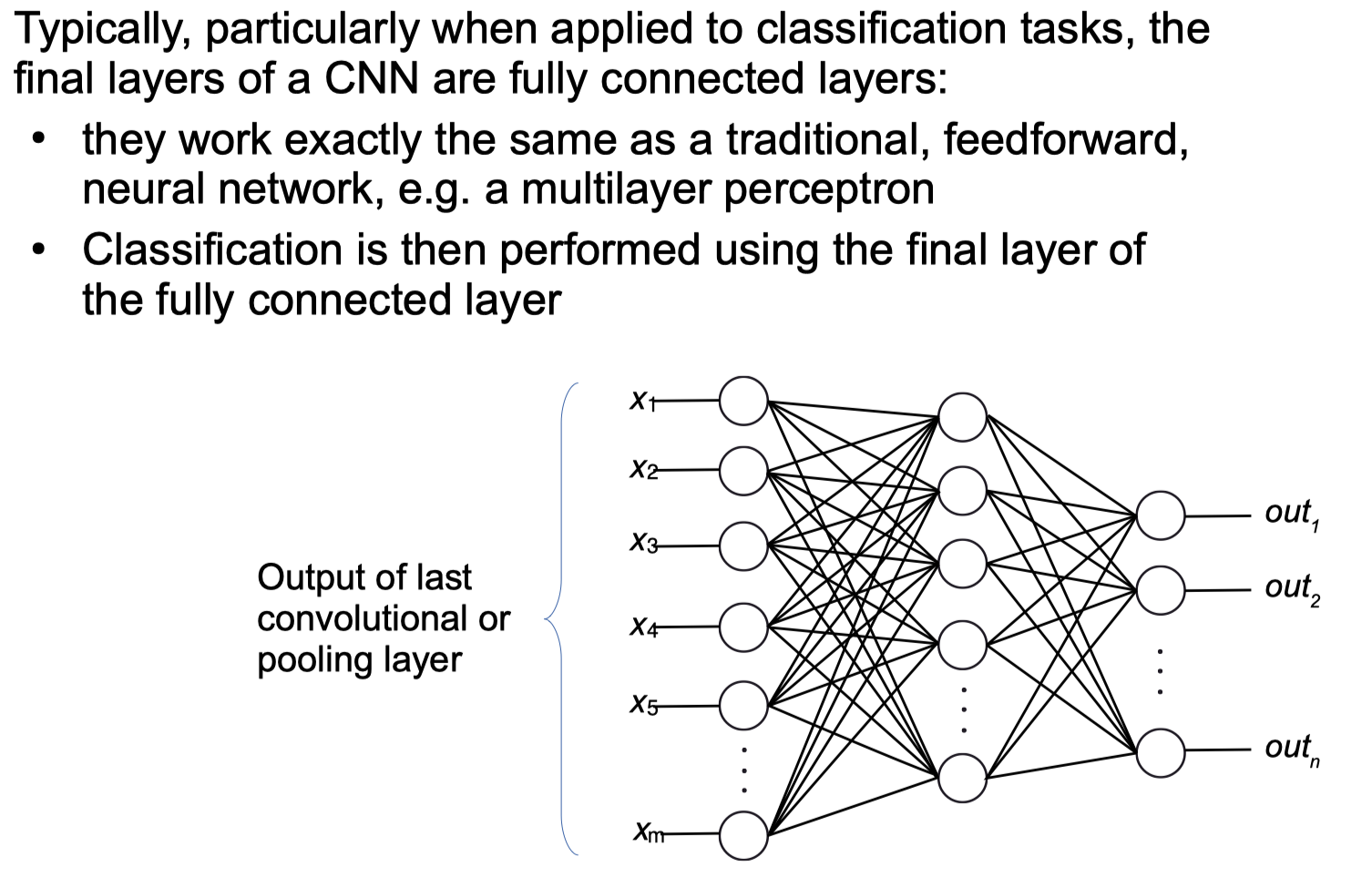
Fully Connected Layers

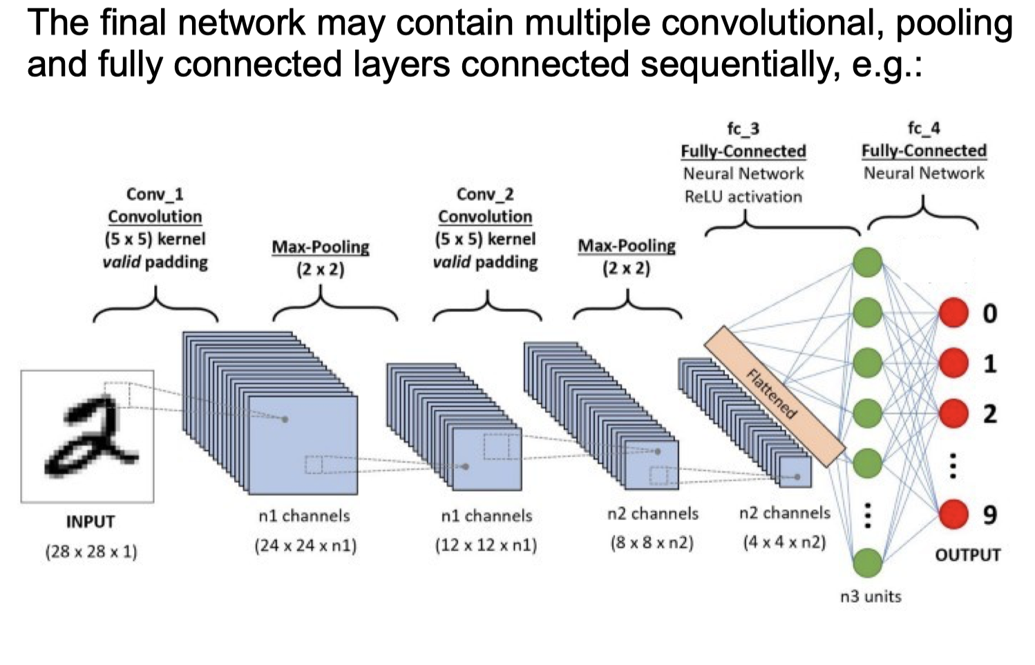
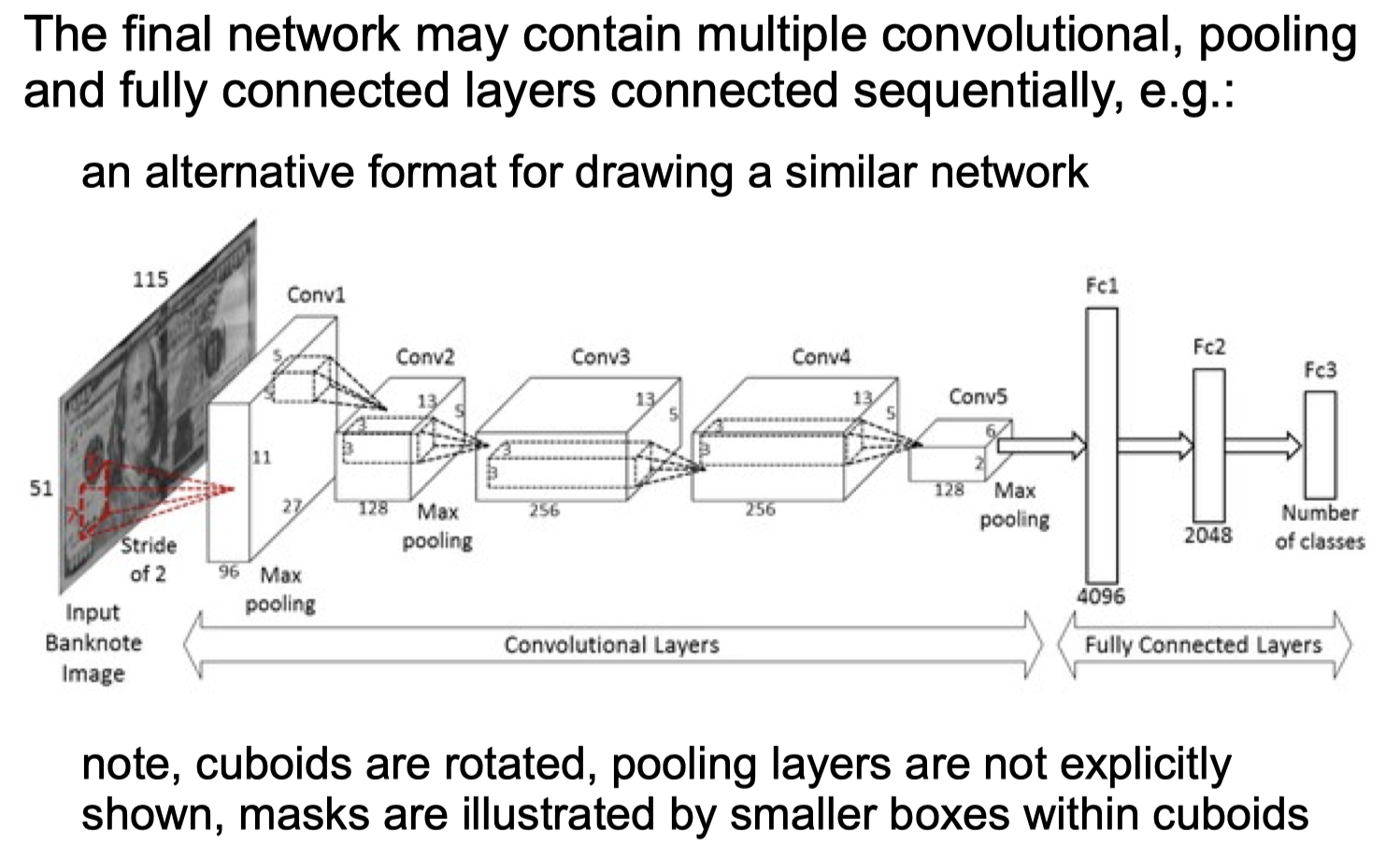
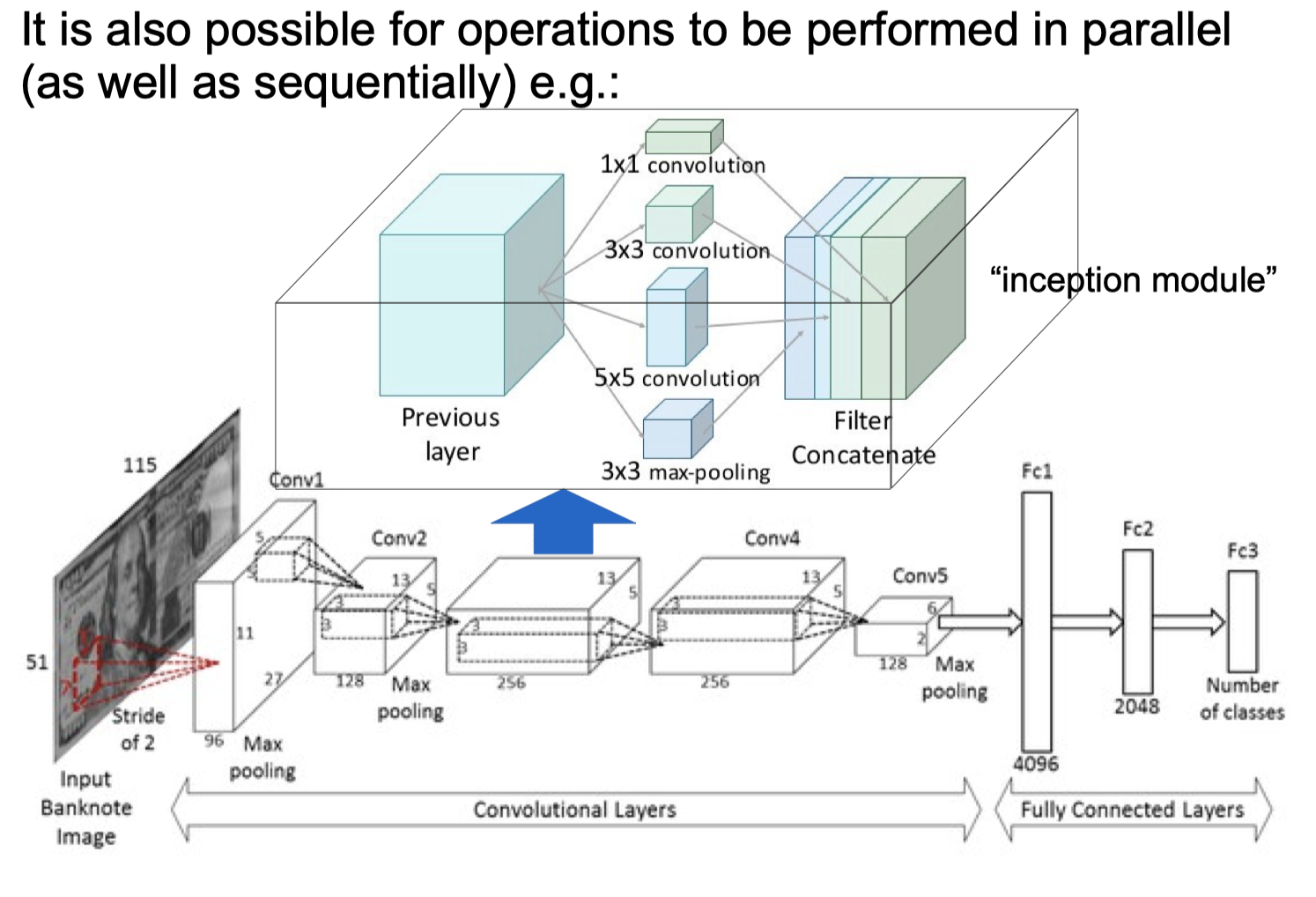
final network

Limitations of Deep NNs

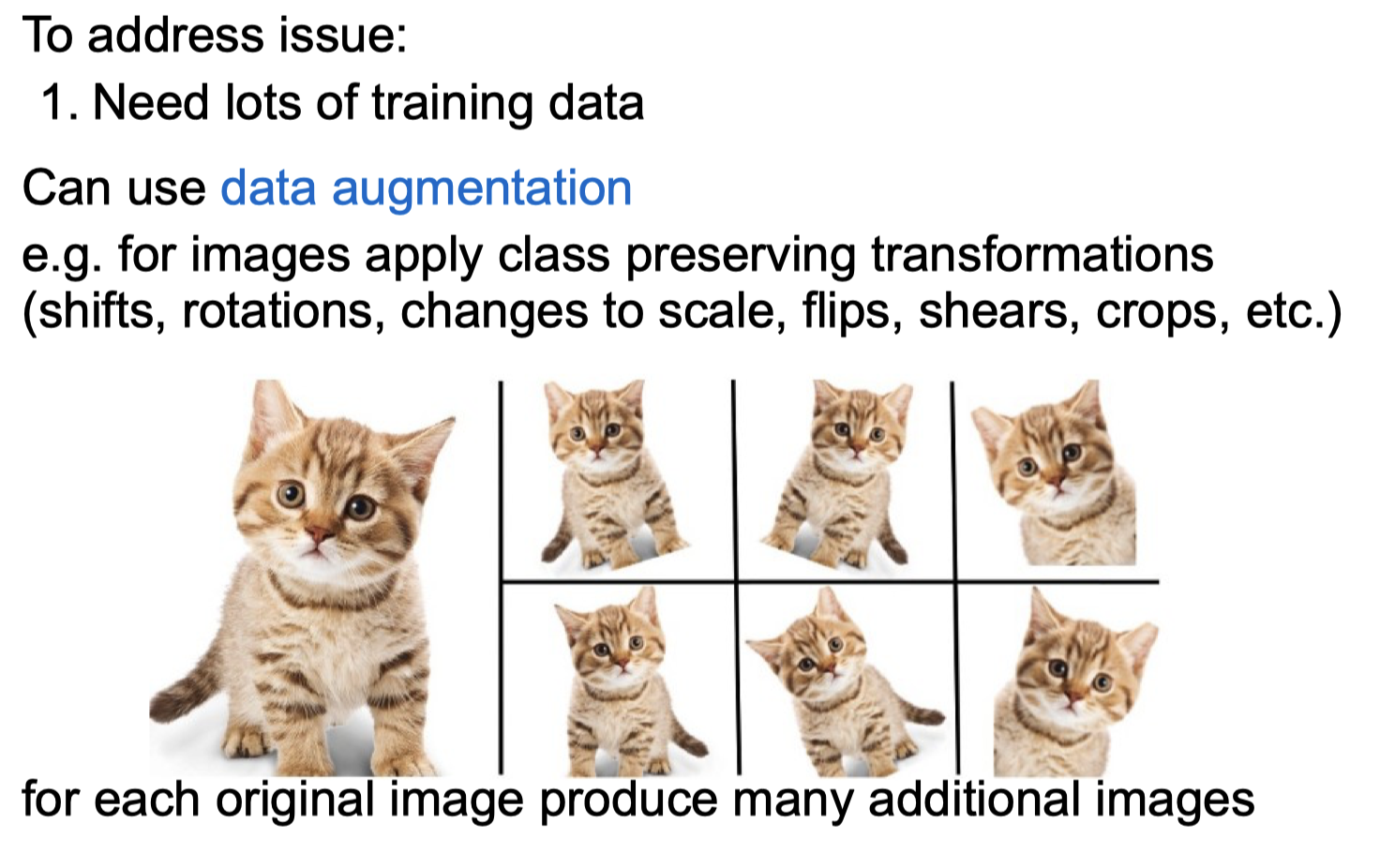
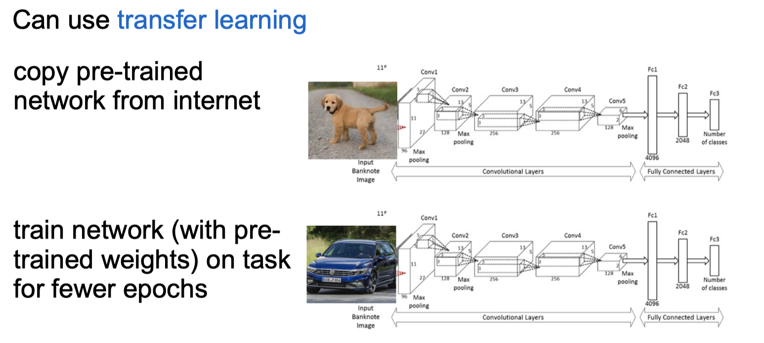
Volume of Training Data

Overfitting

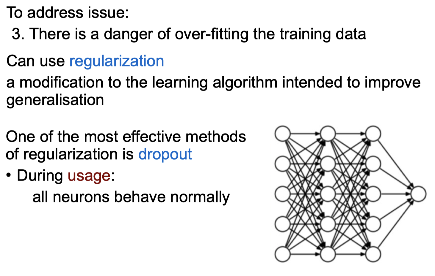
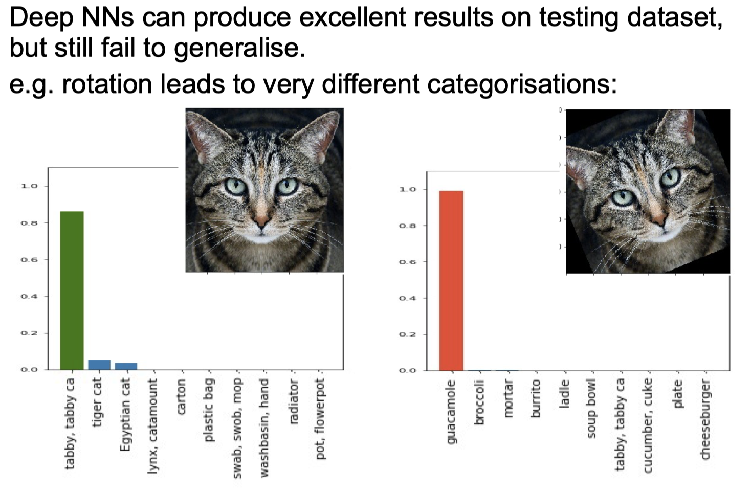
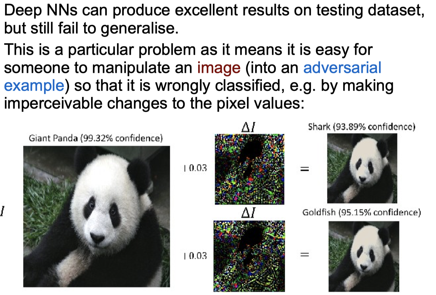
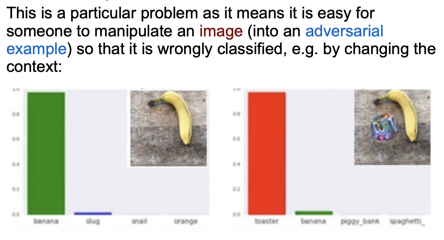
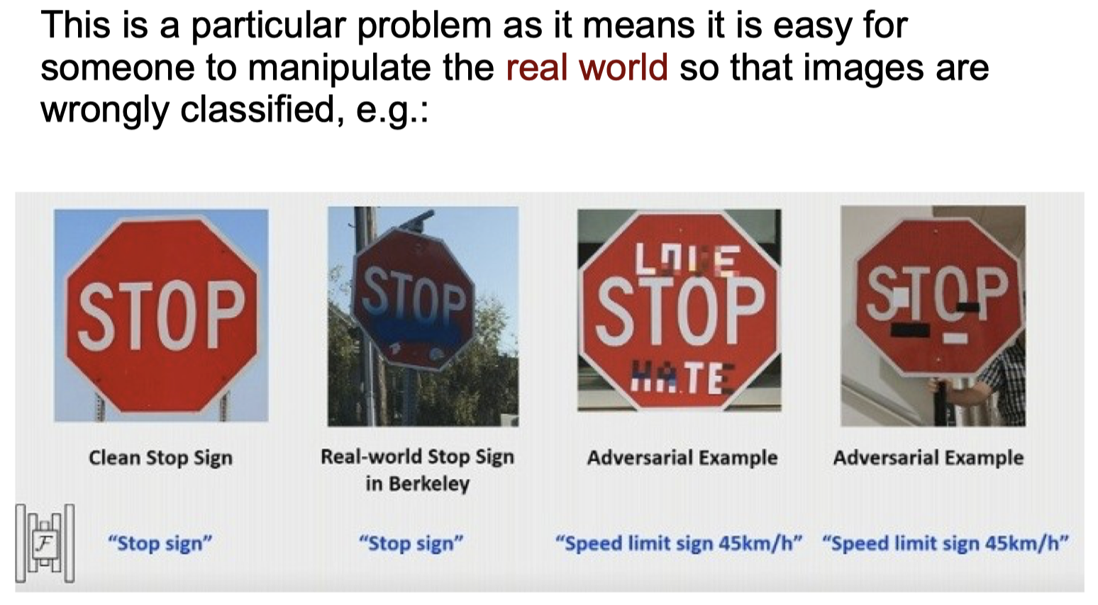
Failure to Generalise