Introduction to Deep Learning

Deep Learning: Introduction to Deep Learning

Here is my Deep Learning Full Tutorial!

Improving Performance

To improve performance, we might

• add more features
• collect more data
• use a model with more parameters (to define a more complex decision boundary)

These choices interact:

• Increasing the number of features → need more data to avoid overfitting
• known as the “curse of dimensionality”
• Increasing the number of parameters → need more data to avoid overfitting
• known as “bias/variance trade-off”

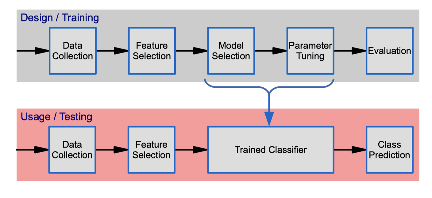
The Classifier Design Cycle

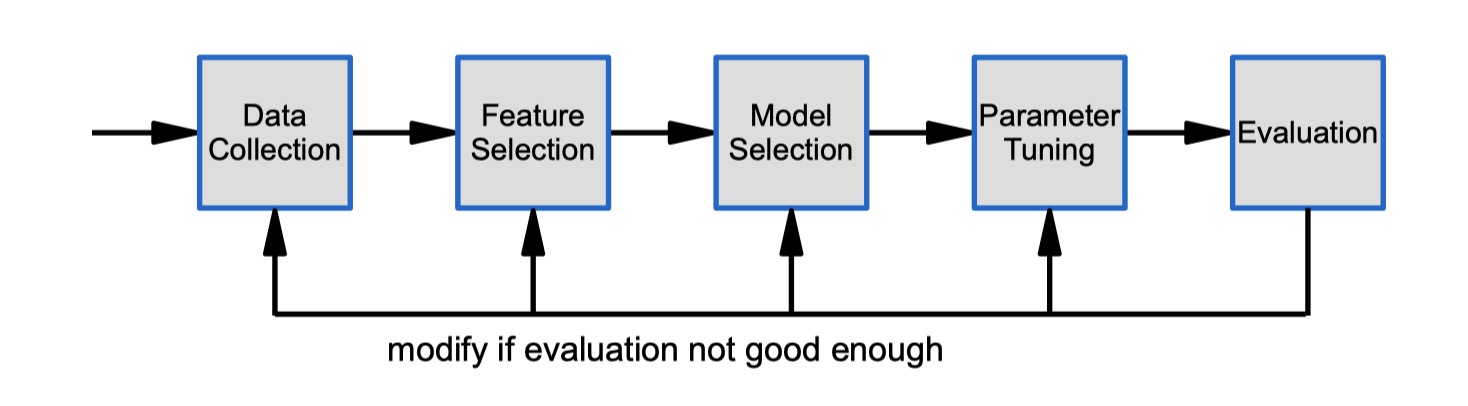
Data collection

Design Considerations:

• What data to collect?

What data is it possible to obtain? What data will be useful?

• How much data to collect?

– need representative set of examples for training and testing the classifier

Data Sources

• One or more transducers (e.g. camera, microphone, etc.) extract information from the physical world.
• Data my also come from other sources (e.g. databases, webpages, surveys, documents, etc.).

Data Cleansing

• Data may need to be preprocessed or cleaned (e.g. segmentation, noise reduction, outlier removal, dealing with missing values).
• This provides the “input data”.

Then input data

This module will:

• Assume that we have the input data
• Concentrate on the subsequent stages

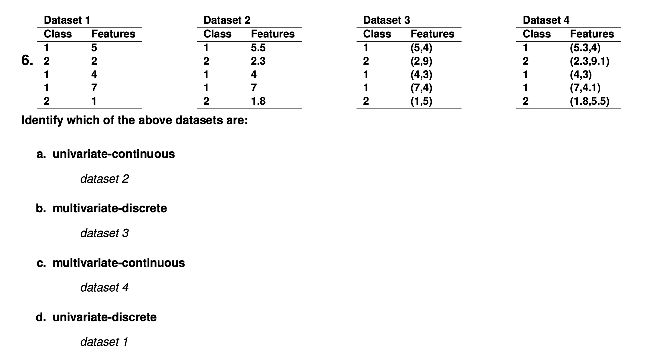
Data is classified as:

• discrete (integer/symbolic valued) or continuous (real/continuous valued).
• univariate (containing one variable) or multivariate (containing multiple variable).

Feature Selection

Design Considerations:

• What features are useful for classification? Knowledge of the task may help decide

Select features of the input data:

• A feature can be any aspect, quality, or characteristic of the data.
• Features may be discrete (e.g., labels such as “blue”, ”large”) or continuous (e.g., numeric values representing height, lightness).
• Any number of features, d, can be used. The selected features form a “feature vector”

Each datapoint/exemplar/sample is represented by the chosen set of features.

• The combination of d features is a d-dimensional column vector called a feature vector.
• The d-dimensional space defined by the feature vector is called the feature space.
• a collection of datapoints/feature vectors is called a dataset.
• datapoints can be represented as points in feature space; the result is a scatter plot.

Model Selection

A model is the method used to perform the classification Design Considerations:

What sort of model should be used?

• e.g. Neural Network, SVM, Random Forest, etc.

Different models will give different results

• However, the only way to tell which model will work best is to try them.

Parameter Tuning

The model has parameters which need to be defined Design Considerations:

● How to use the data to define the parameters?

– There are many different algorithms for training classifiers (e.g. gradient descent, genetic algorithms)

● What parameters to use for the training algorithm?

– These are the hyper-parameters

Need to find parameter values that give best performance (e.g. minimum classification error) ● For more complex tasks exhaustive search becomes impractical

Evaluation

Design Considerations:

• What is criteria for success?

– There a many different metrics that can be used

• e.g. error rate, cost, f1 -score, etc.

– We use “performance” as a general term

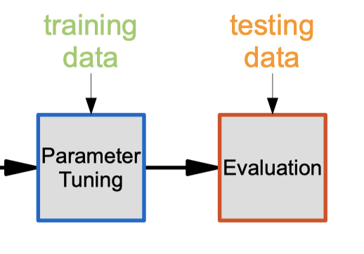
• Evaluation results my vary depending on how the dataset is split.
• A better estimate of performance can be obtained by using multiple (k) splits and averaging results (called “k-fold cross-validation”):

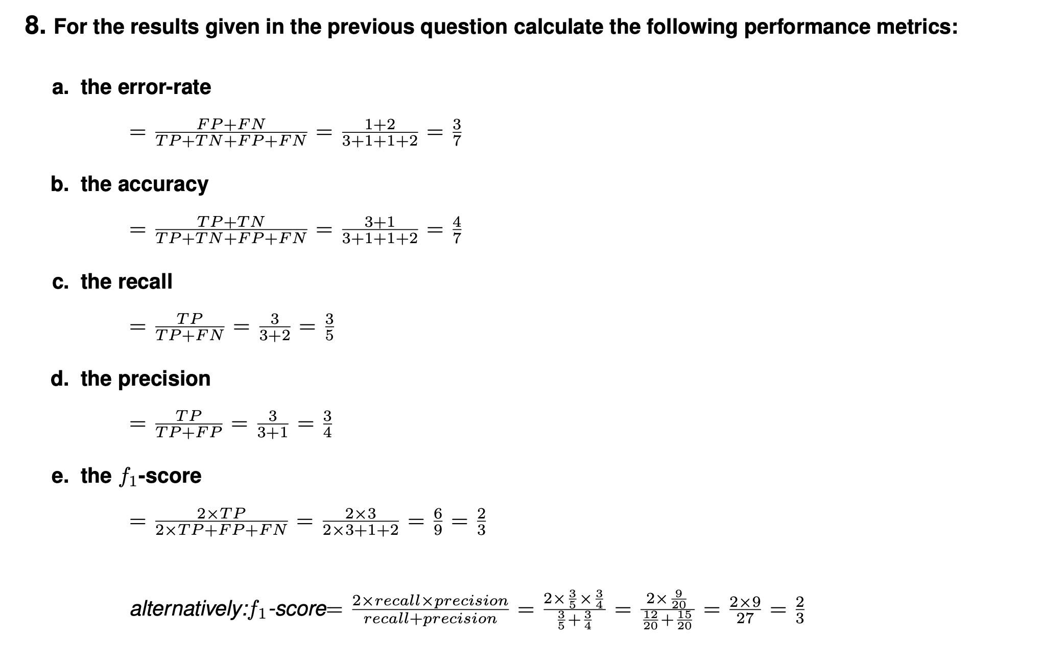
Simplest metric to measure performance is error-rate: The same metric can be expressed as:

● % error (=100xerror-rate) (0 is optimal), or

● accuracy (=1-error-rate) (1 is optimal), or

● % accuracy or % correct (=100-%error) (100 is optimal)

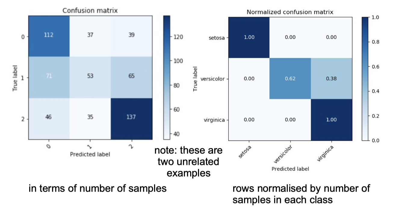
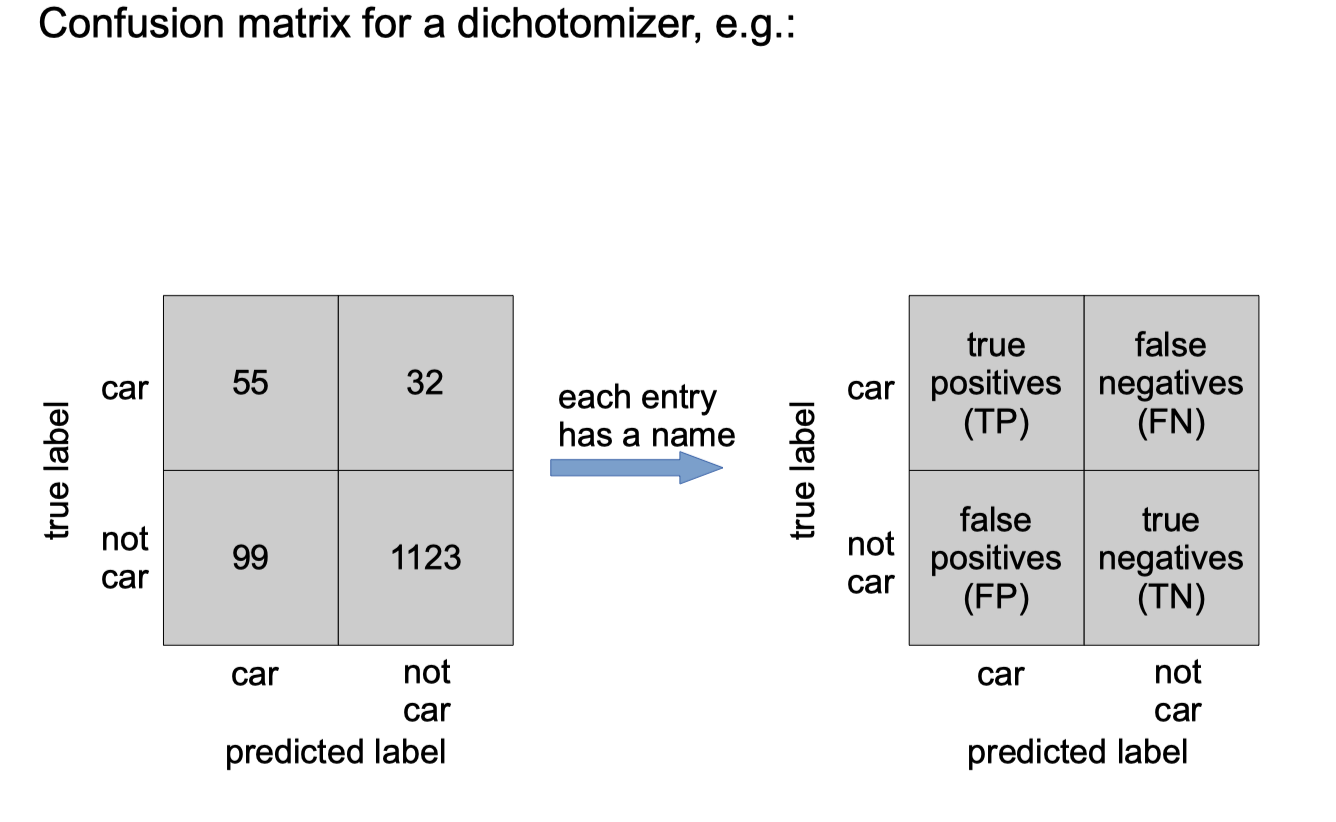
To explore where the prediction errors come from, we can create a confusion matrix, e.g.:

If there are only two classes, then classifier is called a dichotomizer.

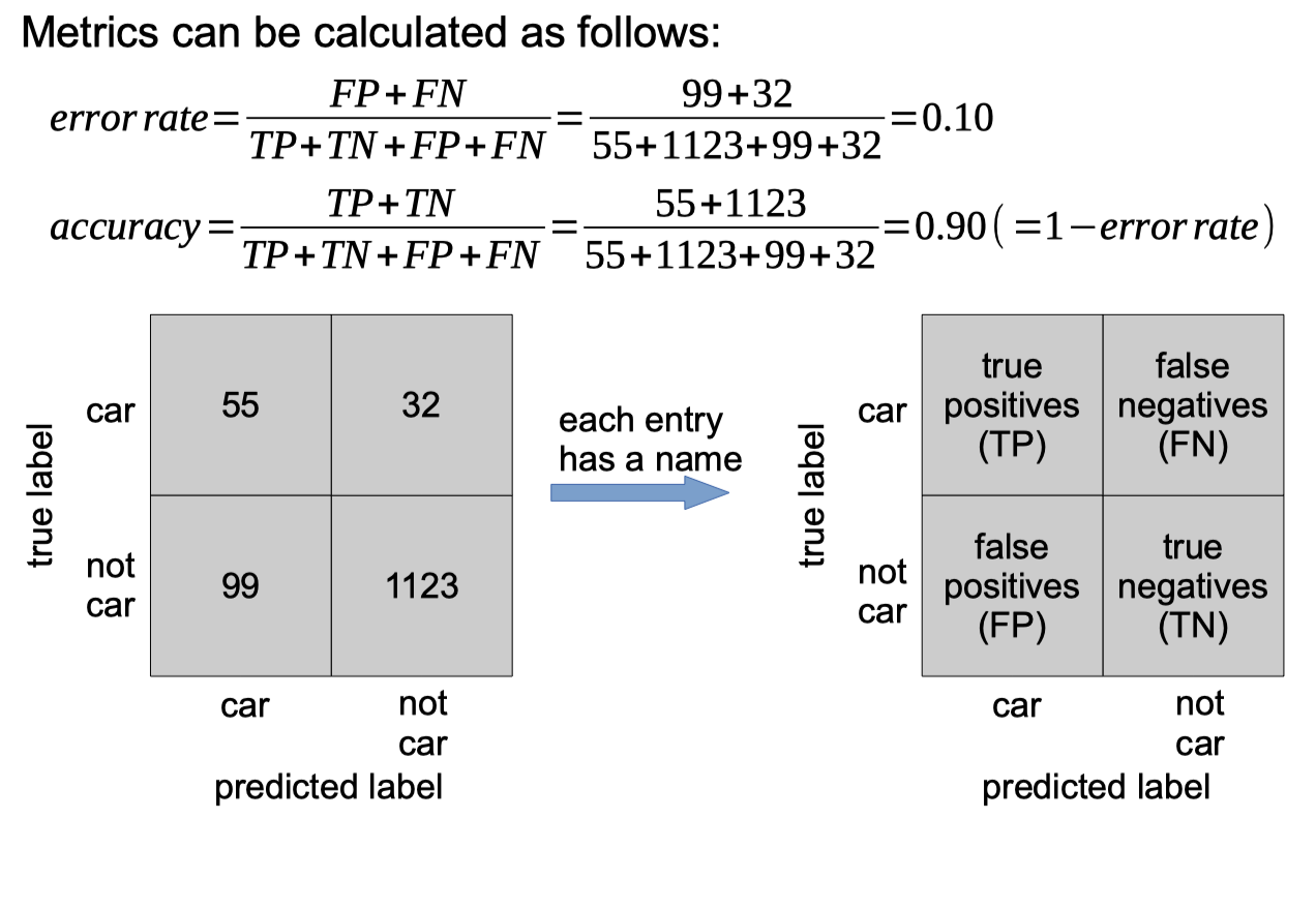
error rate would improve if classifier always predicted “no car” (i.e. if classifier ignored the data!)

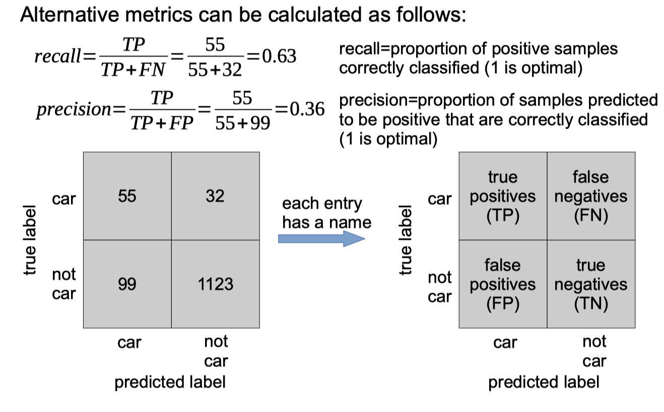
Ignoring the data (by always predicting “false”) leads to poor performance measured with these metrics

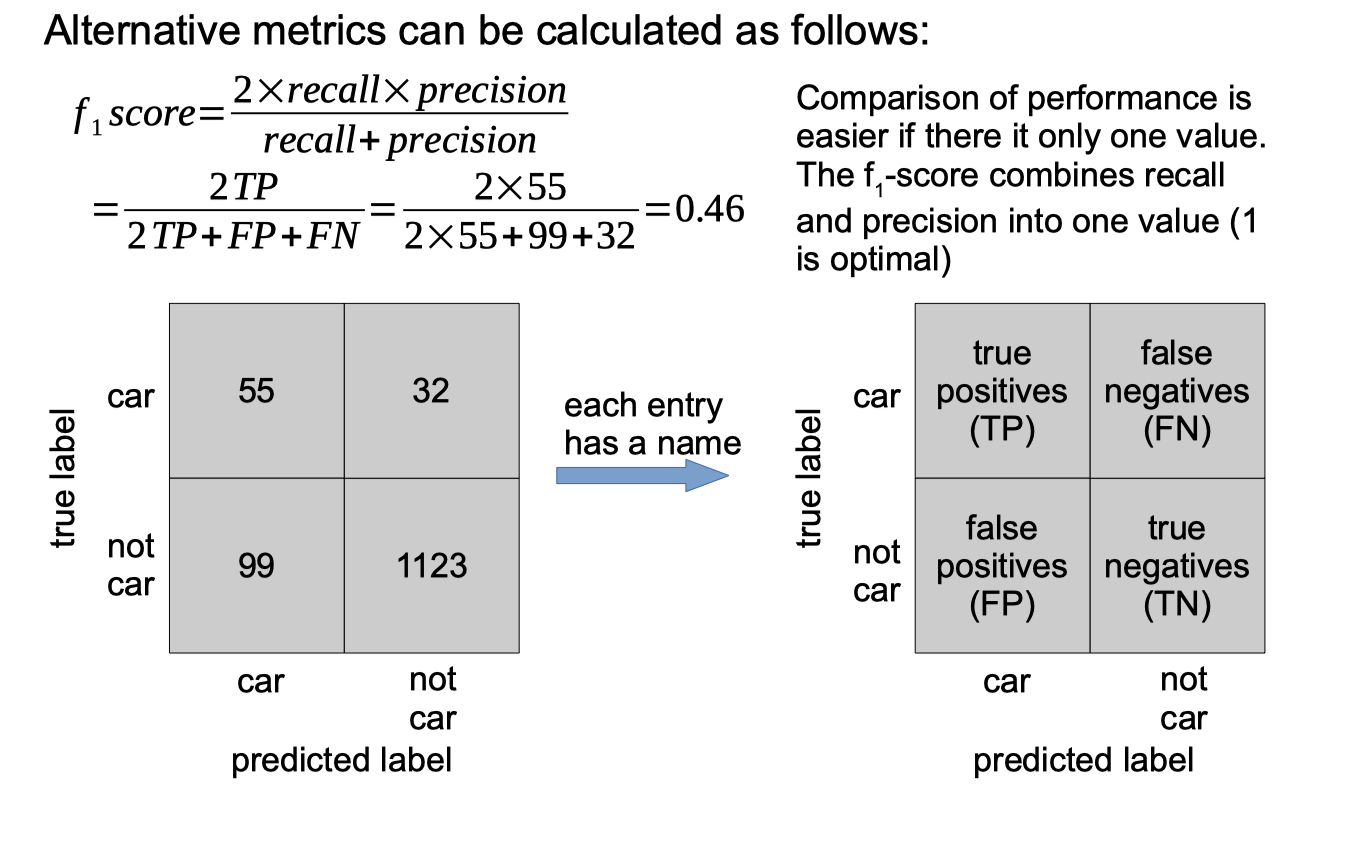
Calculating TP, FP, TN, FN Python code

y =  [1,1,0,1,0,1,1]
y_pred = [1,0,1,1,0,1,0]
TP = 0
TN = 0
FP = 0
FN = 0
for index in range(len(y)):
    if y_pred[index] == 1:
        if y[index] == 1:
            TP += 1
        else:
            FP +=1
    if y_pred[index] == 0:
        if y[index] == 0:
            TN += 1
        else:
            FN += 1
print('TP:',TP,'FP',FP,'TN',TN,'FN',FN)

Output

TP: 3 FP 1 TN 1 FN 2

Calculating error-rate, accuracy, recall, precision, f1 score Python code

from prettytable import PrettyTable
from fractions import Fraction
error_rate = Fraction(FP+FN,TP+TN+FP+FN)
accuracy = Fraction(TP+TN,TP+TN+FP+FN)
recall = Fraction(TP,TP+FN)
precision = Fraction(TP,TP+FP)
f1_score = Fraction(2*TP,2*TP+FP+FN)
result = PrettyTable()
result.field_names = ['error-rate','accuracy','recall','precision','f1_score']
result.add_row([error_rate,accuracy,recall,precision,f1_score])
print(result)

Output

+------------+----------+--------+-----------+----------+
| error-rate | accuracy | recall | precision | f1_score |
+------------+----------+--------+-----------+----------+
|    3/7     |   4/7    |  3/5   |    3/4    |   2/3    |
+------------+----------+--------+-----------+----------+

Learning

Learning is acquiring and improving performance through experience.

Pretty much all animals with a central nervous system are capable of learning (even the simplest ones).

We want computers to learn when it is too difficult or too expensive to program them directly to perform a task.

Get the computer to program itself by showing examples of inputs and outputs.

We will write a “parameterized” program, and let the learning algorithm find the set of parameters that best approximates the desired function or behaviour.

Supervised learning

Regression

● Outputs are continuous variables (real numbers).

● Also known as “curve fitting” or “function approximation”.

● Allows us to perform interpolation.

Classification

● Outputs are discrete variables (category labels).

● Aim is to assign feature vectors to classes.

● e.g. learn a decision boundary that separates one class from the other.

Unsupervised learning

Clustering

• Discover “clumps” or “natural groupings” of points in the feature space
• i.e. find groups of exemplars that are similar to each other

Embedding

• Discover a low-dimensional manifold or surface near which the data lives.

Factorisation

• Discover a set of components that can be combined together to reconstruct the samples in the data.

Semi-supervised learning

The training data consists of both labelled and unlabelled exemplars.

i.e. for some samples we have {x, ω} and for all other samples we have {x}.

Particularly useful when the cost of having a human label data is expensive.

Needs specialist learning algorithm that is able to update parameters both when a label is and isn’t provided.

Reinforcement learning

For each input, the learning algorithm makes a decision: ω*=g(x)

A critic, or teacher, compares ω* to the correct answer, and (occasionally) tells the learner if it was correct (reward) or incorrect (punishment).

Learning uses reward and punishment to modify g to increase reward received for future decisions.

instead of a dataset containing {x, ω} pairs, we get {x, g(x), reward/punishment}.

Transfer learning

Train the classifier (with initially random parameters) on one task for which data is abundant.

• i.e. use a dataset containing many {x, ω} pairs.

Train the classifier (with initial parameters pre-trained on 1 st task) on second tasks for which data is less abundant.

• i.e. use a dataset containing {x, ω} pairs.

Expectation is that pre-training the classifier on the first task will help if perform well on the second task.

• 1st task needs to be “similar” to 2nd task.

Hyper-parameters

The learning algorithm will also have parameters:

• More practical algorithms may have many parameters.
• These are called hyper-parameters (to distinguish them from the parameters being learnt by the classifier).
• The choice of hyper-parameters may have a large influence on the performance of the trained classifier.
• Choosing hyper-parameters:
  • exhaustive search (called grid search)
  • learning (called meta-learning)

Deployment